Overview
In this tutorial we’re going to simulate the steady-state stresses of a spinning electric ducted fan in Coreform Flex. But I also want to tell a story, a story that helps explain why we’ve developed Coreform Flex. I know that many readers, especially on this forum, will be familiar with traditional meshing workflows and the pains inherent to it. However I think this exercise will be enlightening even for the experienced analyst, while also demonstrative to the non-analyst who’s wants to understand the issues with traditional meshing.
To this end, I will first demonstrate traditional hex & tet-meshing workflows and then I will show the simulation setup procedure for this fan within Coreform Flex – which we’ll see is a meshing-free workflow that allows us to move immediately to analysis. Because this is a long post, I’ll summarize at the front.
Summary
To build an all-hex mesh on the fan geometry took me approximately 40 hours (though inefficient hours on airplanes, in airports, while watching college football) and required pretty significant defeaturing of stress-relief fillets. An all-tet mesh took me approximately an hour to construct due to some deep bug either with the CAD geometry, Coreform Cubit’s underlying CAD kernel, or mesh algorithms within Coreform Cubit, that I had to work around.
Conversely, within one hour I not only Flex-meshed the fan assembly in Coreform Flex, but I’d also setup, solved, and viewed the simulation results. Furthermore, since I was able to script the entire process in Python, future analyses of different fan geometries could be completed within minutes.
– As a final note before beginning, I ran up against our forum post character and data limits so I’ll be investigating some different forms of providing this (and other) tutorials, which should allow you to replicate tutorials directly in our tools… stay tuned!
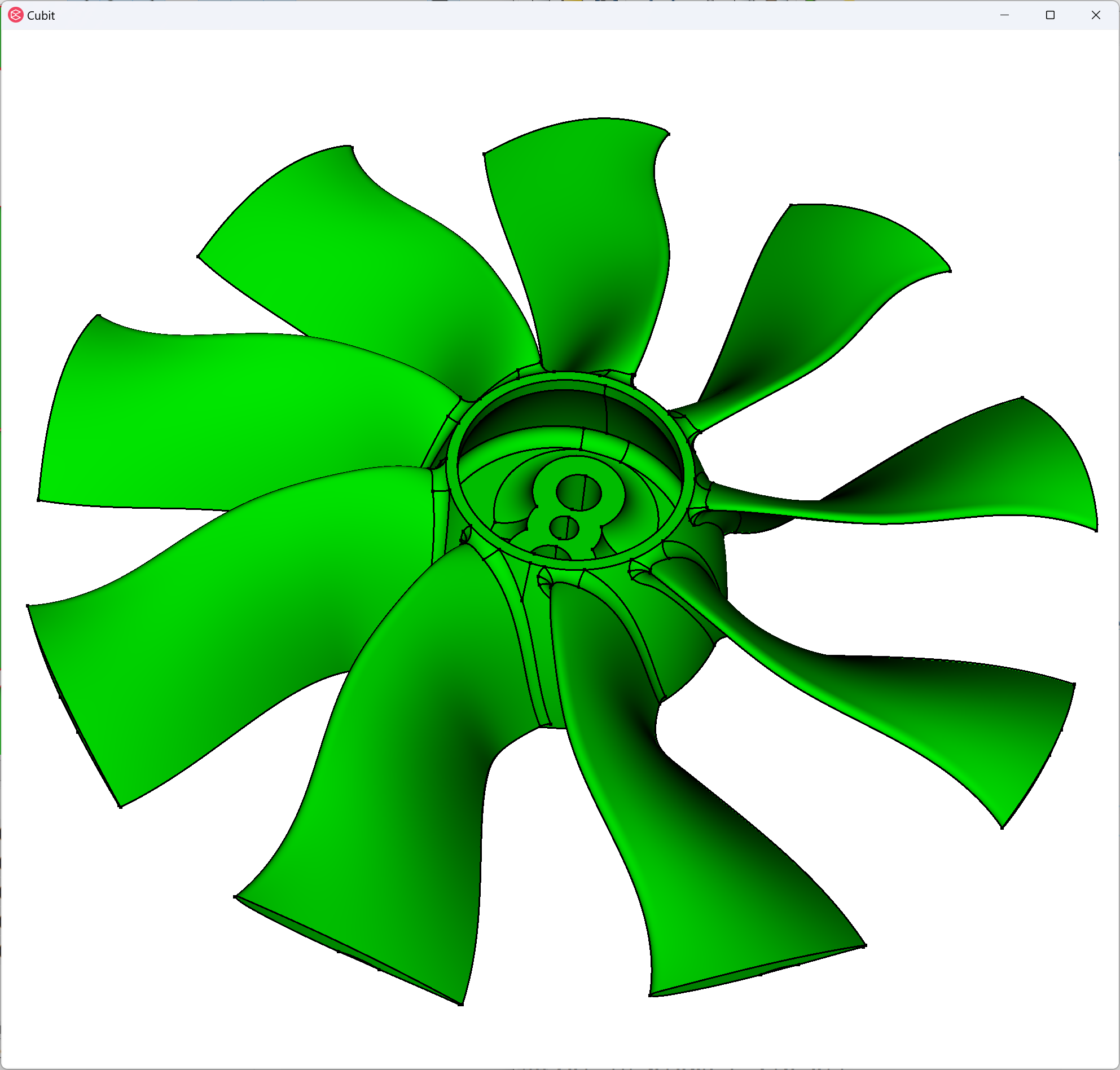
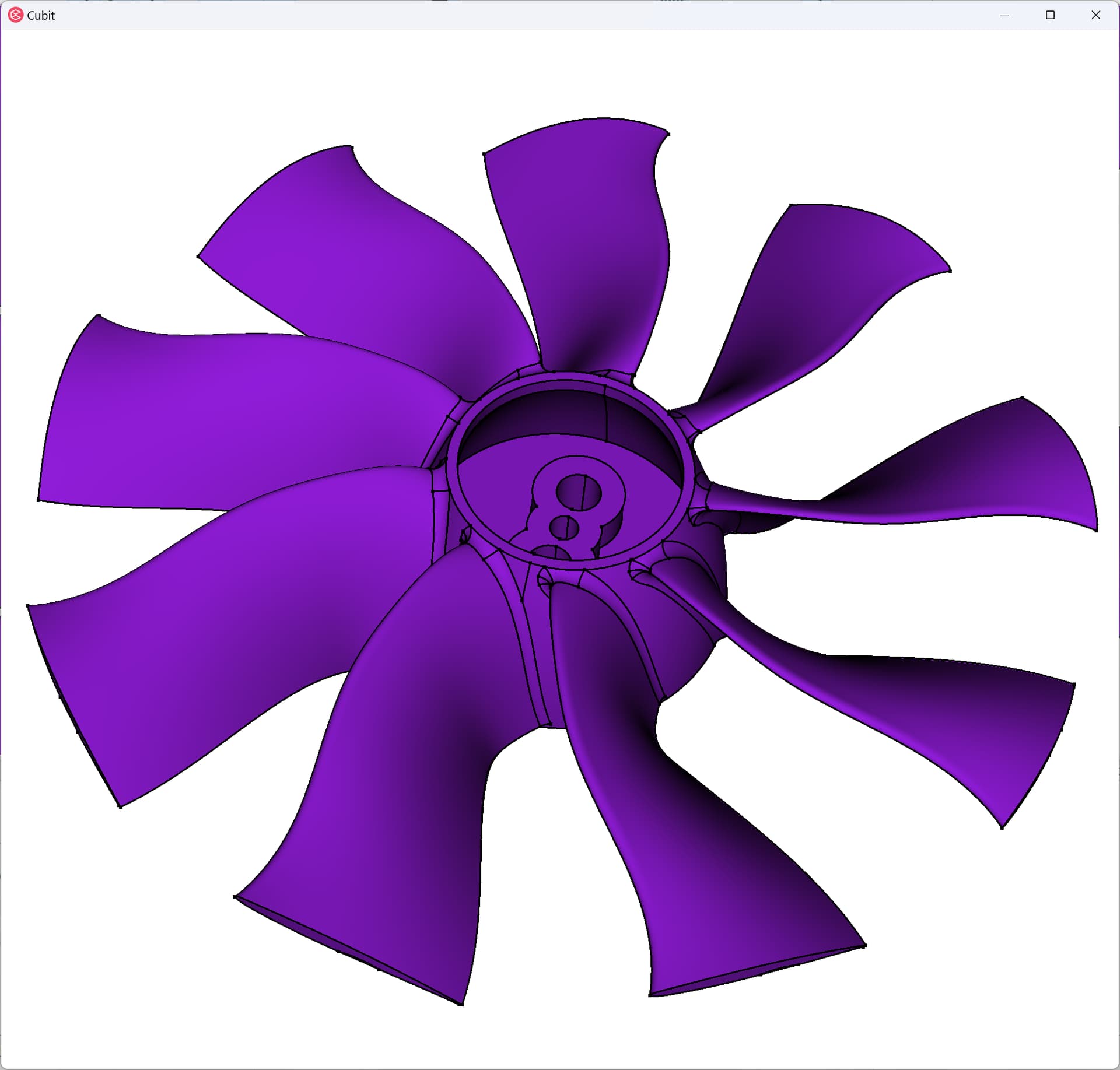
Geometry
The geometry for this simulation comes from this GrabCAD project by the GrabCAD user chris.t-35. Here’s the STEP file for your convenience:
55mm_EDF.STEP (2.0 MB)
Challenges with traditional meshing
I would be remiss if I didn’t first talk about traditional meshing approaches.
Meshing the rotor cone
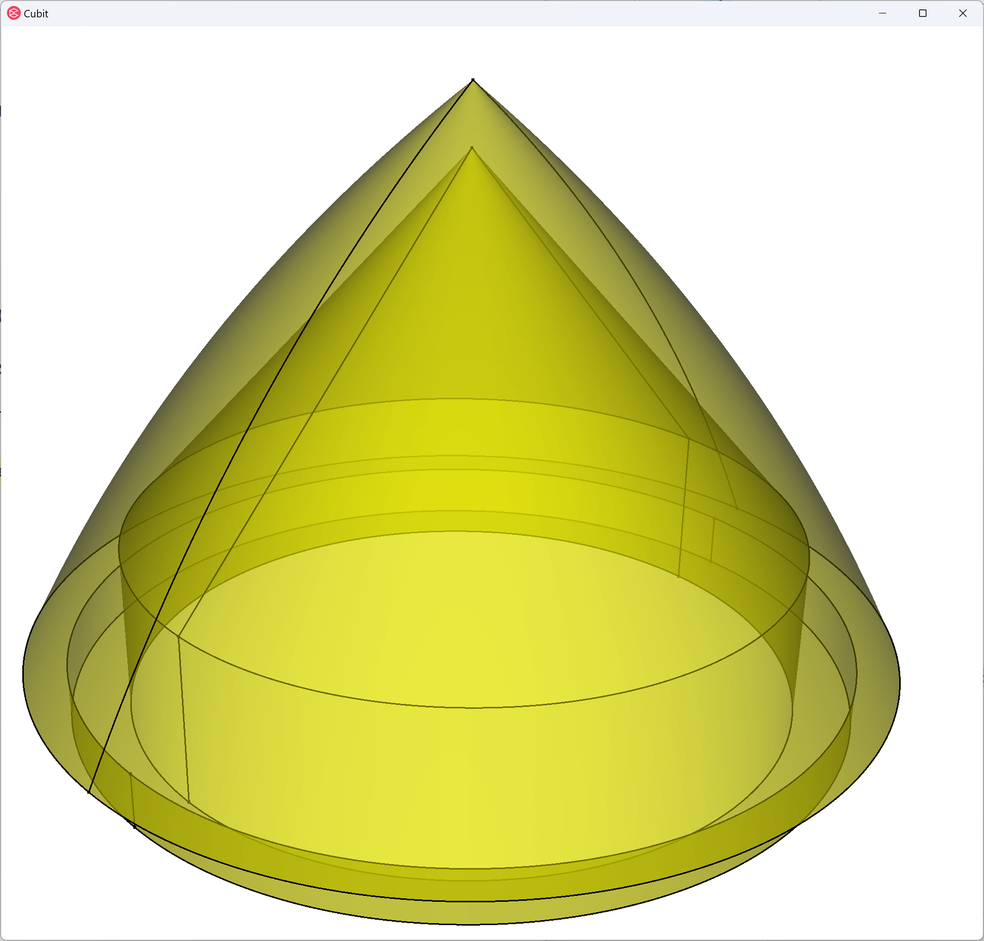
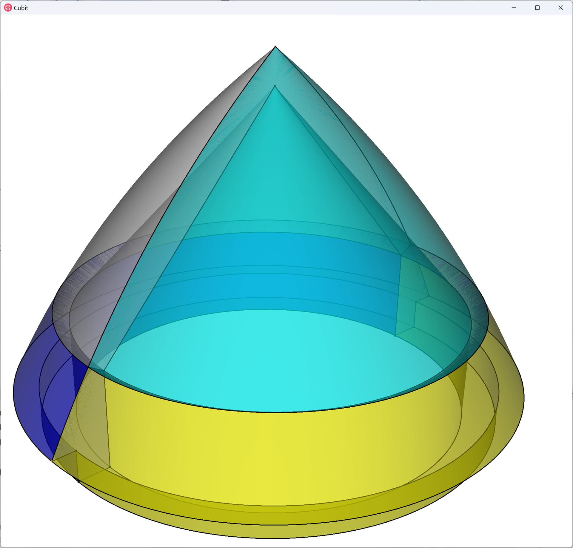
The rotor cone is fairly straightforward to mesh. We begin by recognizing that we can decompose the cone into two regions, the inner core and the outer rim, that are independently hex-meshable. We can use Coreform Cubit’s extensive geometry creation and webcutting tools to decompose it into these two major regions:
reset

# Import geometry
import step "/Path/To/55mm_EDF.STEP" heal

# Assign blocks for assembly management
block 1 vol 1
block 2 vol 2

block 1 name "fan"
block 2 name "rotor_cone"

# Mesh the rotor cone
## Cut into outer rim and inner core regions
create vertex on curve 321  close_to vertex 206
create curve vertex 206 214
sweep curve 338  along curve 337
webcut volume 2  with sheet extended from surface 129

## Cleanup temporary tool geometry
delete body 3
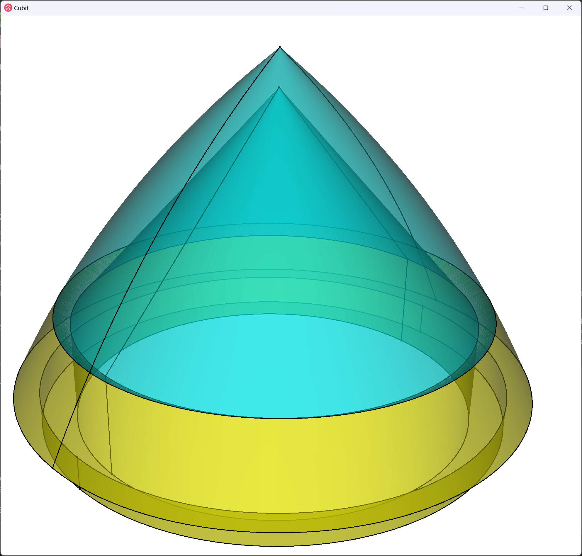
A limitation in Coreform Cubit is that it doesn’t support “many (surface) to many (surface)” sweeps, so we’ll cut both volumes along a plane normal to the outer curve at the vertex locations of the radial curves (the curves emanating from the tip of the cone):
webcut volume in block 2 with plane normal to curve 333 close_to vertex 203
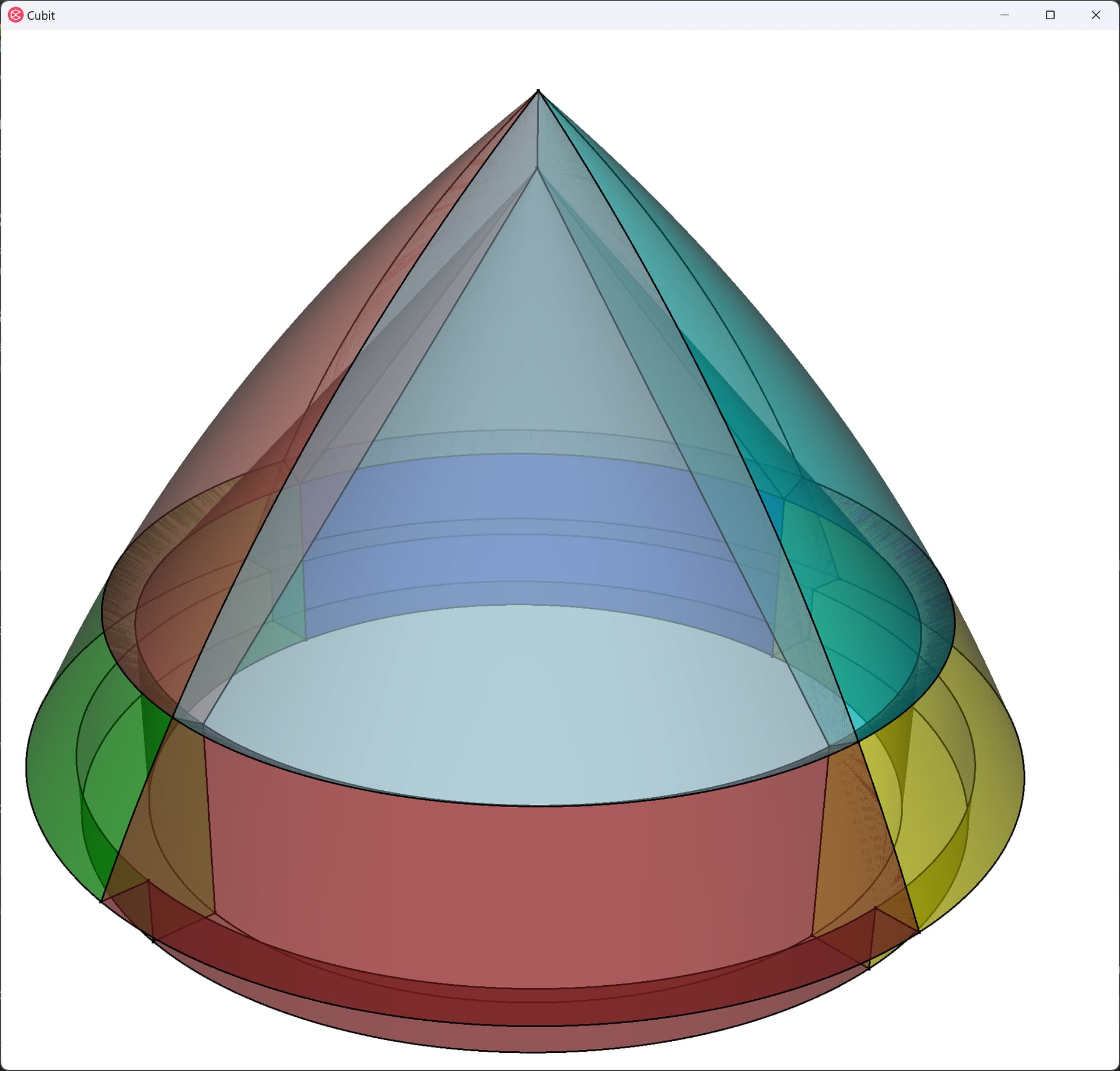
And then we cut these two halves in half again, using a plane normal to the midpoint of the outer curve(s):
webcut volume in block 2 with plane normal to curve 333 fraction .5 from start
We then merge these volumes back together, to ensure a contiguous mesh, and mesh the rotor cone:
merge vol in block 2

volume in block 2 size 1
volume in block 2 scheme auto
mesh volume in block 2
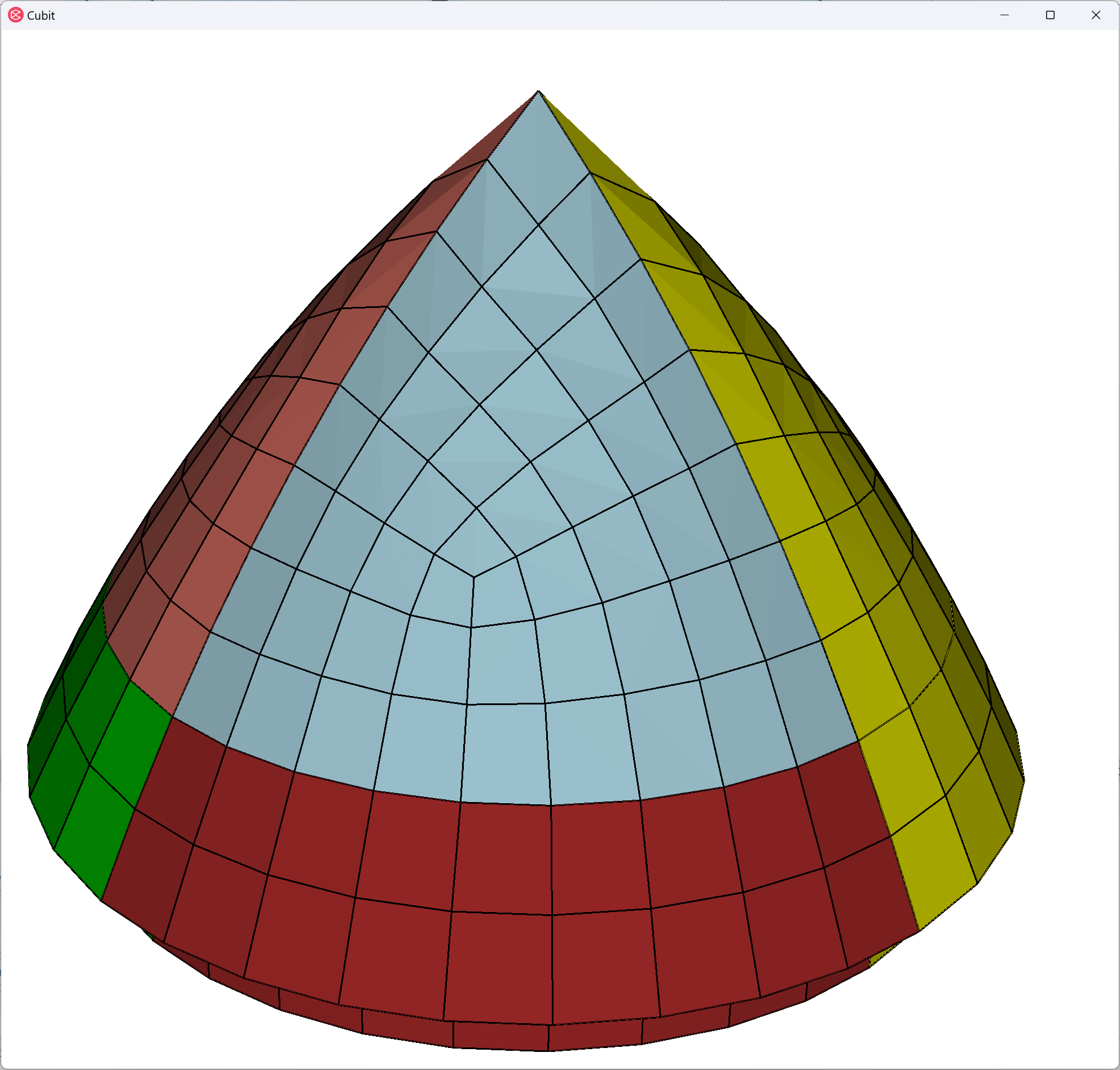
Easy enough. About one minute for me to mesh when I first got this model, I’ve had a lot of practice!
Here’s the full journal file to this point:
#!cubit
reset

# Import geometry
import step "/Path/To/55mm_EDF.STEP" heal

# Assign blocks for assembly management
block 1 vol 1
block 2 vol 2

block 1 name "fan"
block 2 name "rotor_cone"

# Mesh the rotor cone
## Cut into outer rim and inner core regions
create vertex on curve 321  close_to vertex 206
create curve vertex 206 214
sweep curve 338  along curve 337
webcut volume in block 2  with sheet extended from surface 129

## Cleanup temporary tool geometry
delete body 3

## Partition the rotor cone for meshability
webcut volume in block 2 with plane normal to curve 333  close_to vertex 203
webcut volume in block 2 with plane normal to curve 333  fraction .5 from start

## Enforce contiguous mesh
merge volume in block 2

## Assign mesh scheme and generate mesh
volume in block 2 size 1
volume in block 2 scheme auto
mesh volume in block 2
Meshing the fan
Now comes the hard part: meshing the fan. Now, I’ve spent nearly 40 hours trying to hex-mesh this fan. First I have to compromise and remove the fillets on the interior of the fan:
remove surface 117 115 116 118  extend
Surface 110  copy nomesh
sweep surface 110   perpendicular distance 1
remove surface 4 114 113 112 extend
webcut Volume 1 tool Body 11
delete Body 11
delete volume 1
So that I can again separate the fan into an inner core region an an outer “ring”
webcut volume 12 sweep surface 198 perpendicular inward through_all

Now, since we know the inner region is now meshable, let’s turn our attention to the outer “ring”. A trick I often do with objects with rotational symmetry is: chop it into a symmetric section, make the subsection hex-meshable, create rotational pattern of the meshable subsection, imprint and merge:
create vertex on curve 84 86  midpoint
create vertex on curve 242  close_to vertex 107 93 94 80
create curve arc  three vertex 335 337 338
split curve 539  close_to vertex 336 337
create vertex on curve 540  midpoint
create vertex on curve 542  midpoint
create curve vertex 333 345
create curve vertex 334 346
create vertex on curve 543 544  midpoint
create vertex location on surface 59  close_to location at vertex 347
create vertex location on surface 59  close_to location at vertex 348
webcut volume 13  with plane vertex 333  vertex 349  vertex 345
webcut volume 13  with plane vertex 334  vertex 350  vertex 346
delete volume 13, 15
delete curve all
delete vertex all
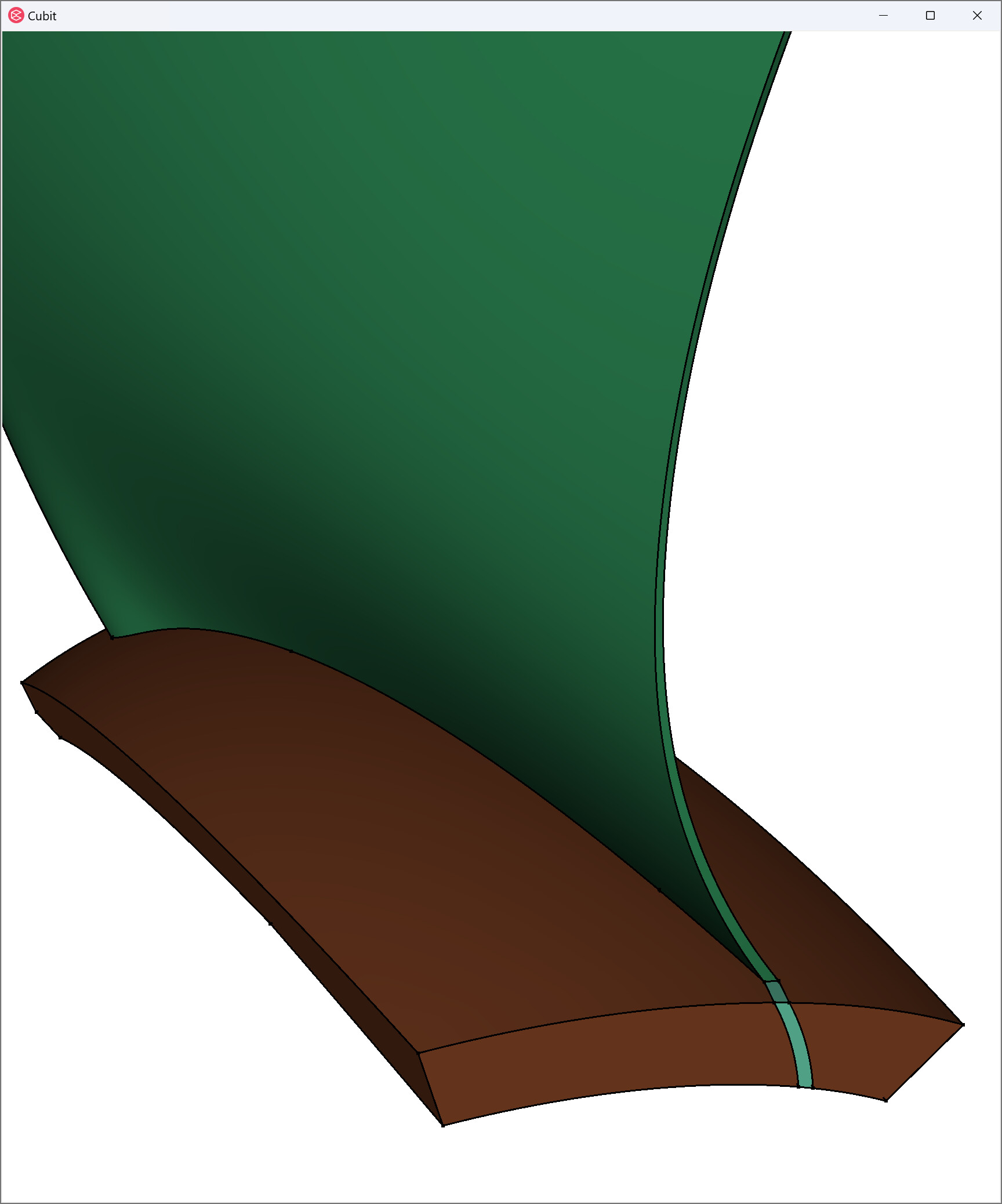
Which produces this symmetric section:
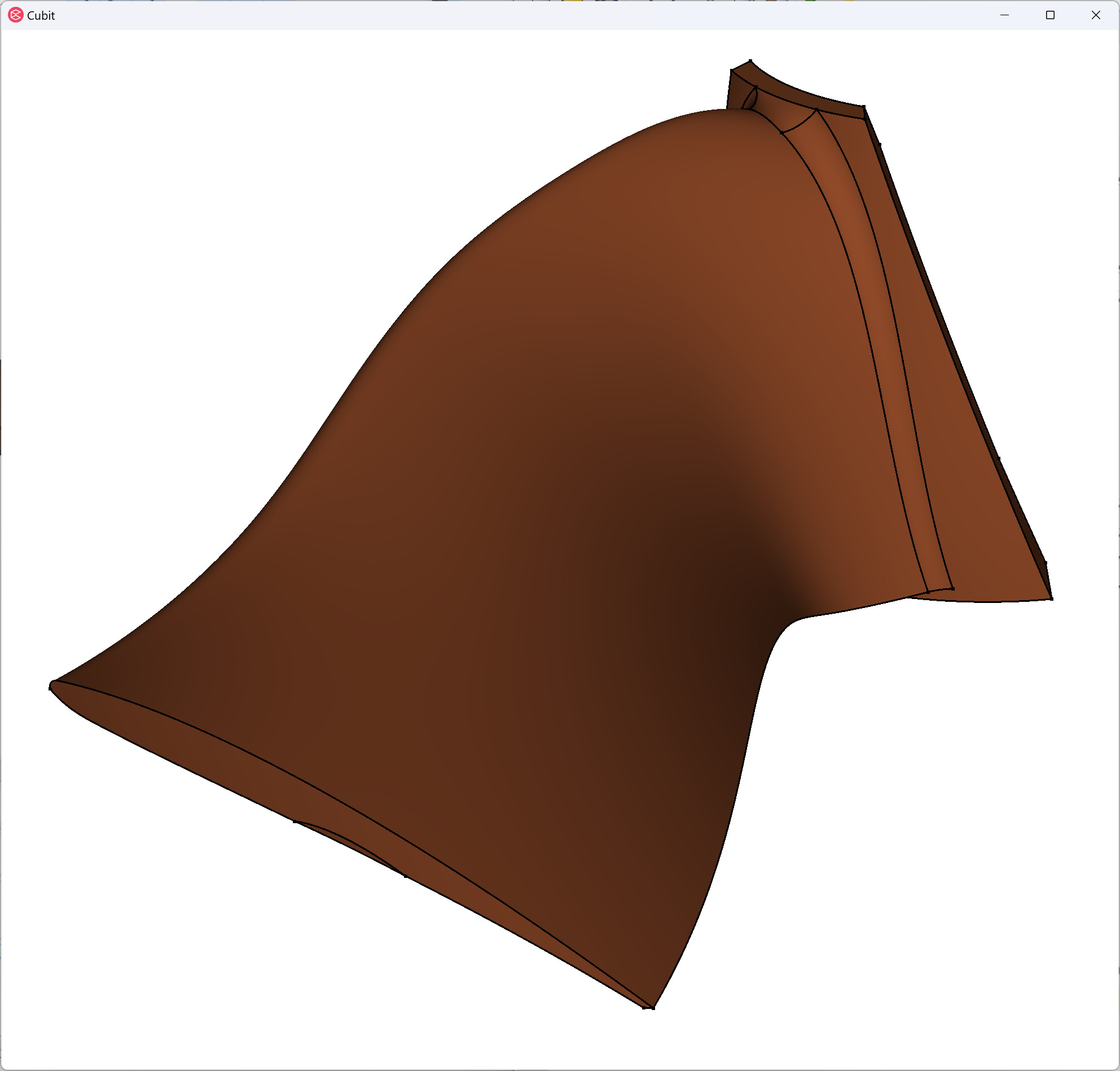
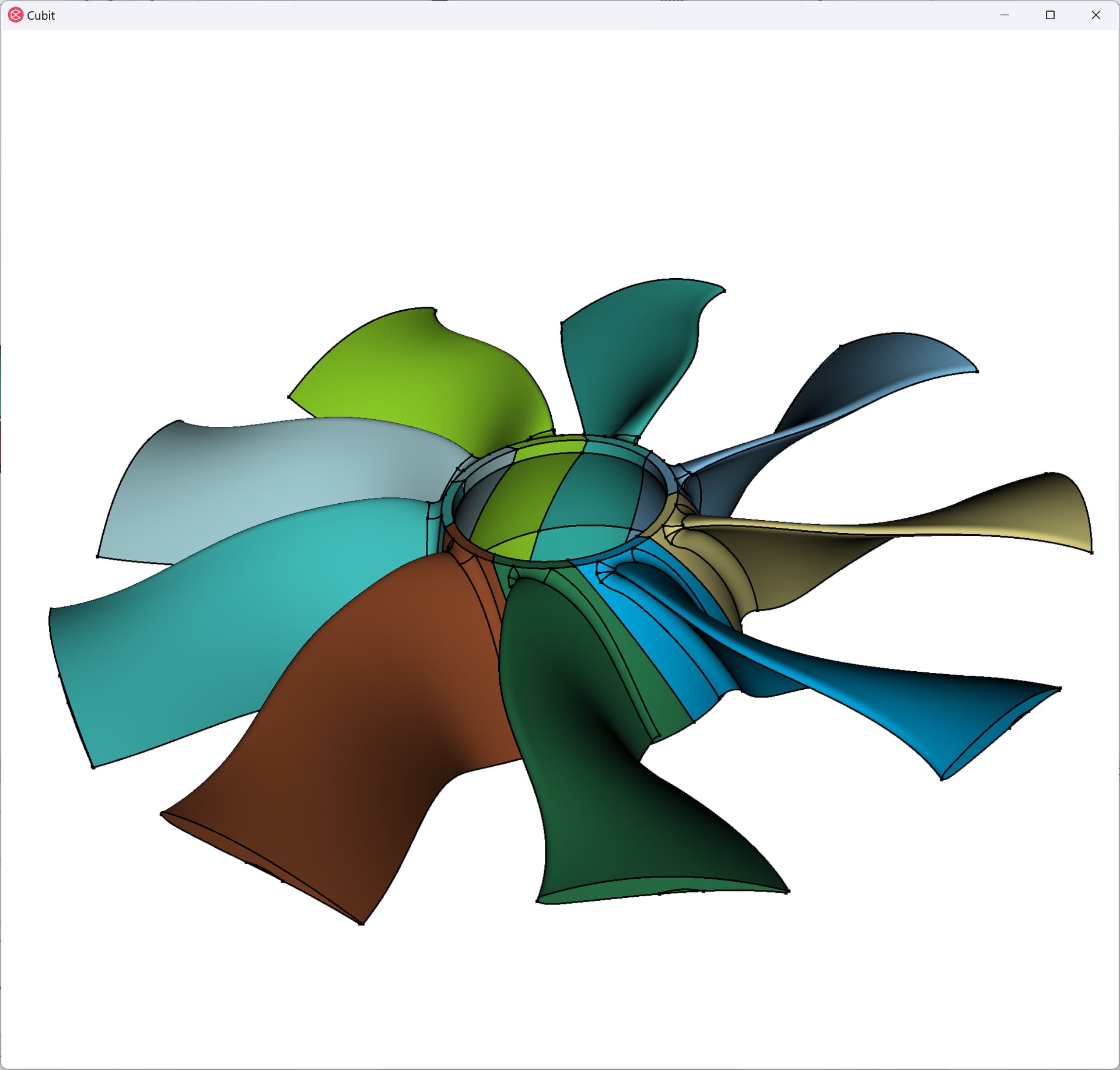
Which we can “preview” how this piece would be rotationally instanced:
create vertex center curve 660
create vertex center curve 656

#!python
c = cubit.surface(288).center_point()
n = cubit.surface(288).normal_at( c )
cubit.cmd( f"Volume 16  copy reflect origin {c[0]} {c[1]} {c[2]}  direction {n[0]} {n[1]} {n[2]}  nomesh  preview" )

#!cubit
Volume 16  copy rotate 40 about vertex 409 410 repeat 8 nomesh
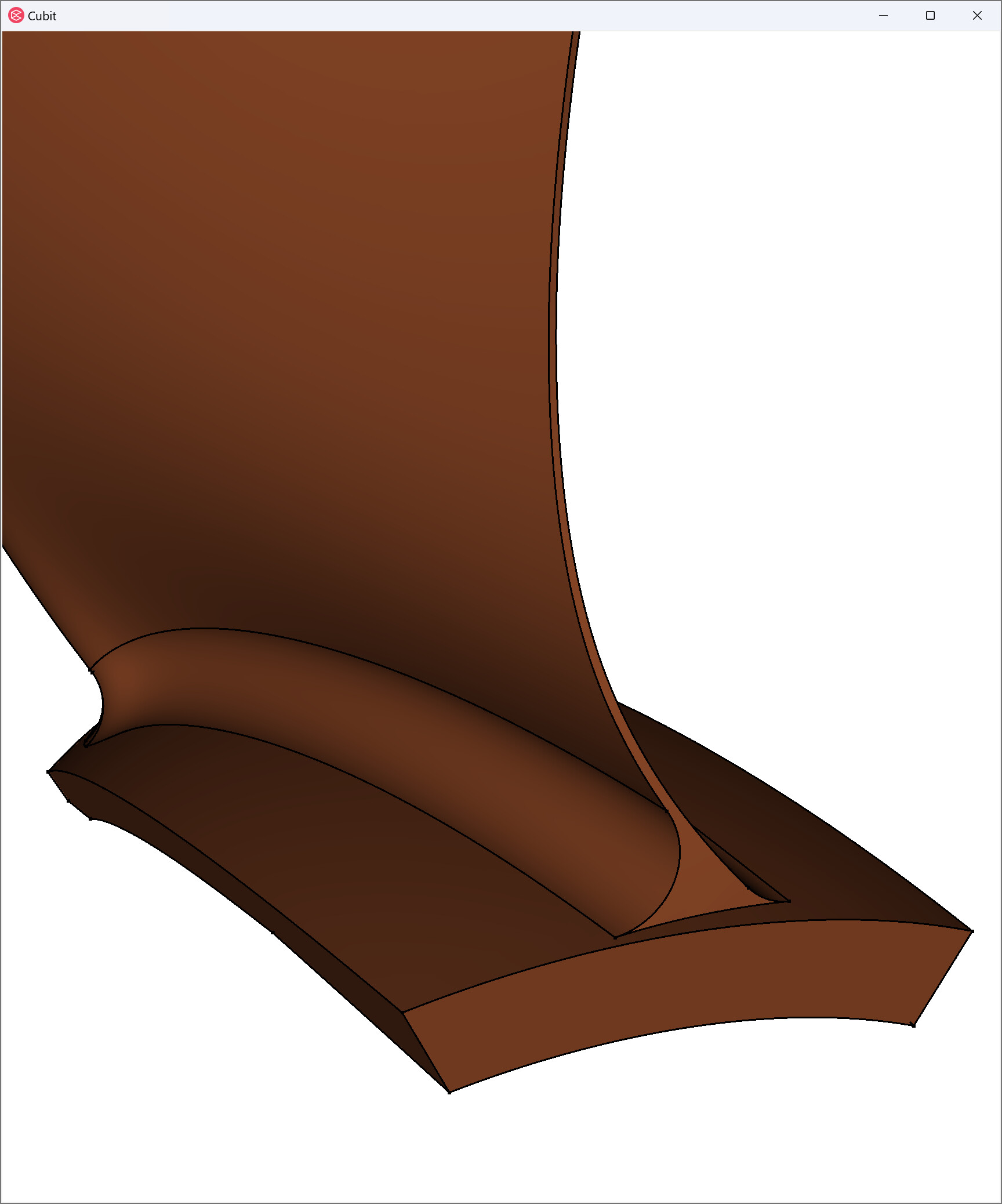
But here is the issue… try as I might… I cannot get an all-hex mesh (of good element quality) on this blade subsection without removing the fillets along the base of the blade. I’ve spent four airplane rides (plus layovers), a few sleepless nights with a newborn, and a few stressful college football games trying to mesh this single blade part. The approaches I’ve attempted to use run into very minor numerical errors during projection that result in bad CAD, but even if my attempts did work, I’m still not convinced the blade would be all-hex meshable due to the large angle of the fillets:
As a challenge to the community, to the first person to build a quality, all-hex mesh on either of the below CAD files that can be “pinwheeled” back to the full fan mesh I will send you a coffee cup with a Coreform Cubit logo and an image of your meshed blade. Note that I will roughly define quality as being a min( Scaled Jacobian ) ≥ 0.25 for the mesh.
single_blade.stp (177.1 KB)
single_blade.sat (316.9 KB)
Instead I remove the fillets and then do some fancy webcutting:
to obtain a mesh of my desired quality:
Great! So I can get a hex-mesh… but at what cost? Not only have I spent many hours producing this mesh, but I’ve also removed potentially critical features from my geometry. I’ll need to proceed with my analysis carefully to understand what the response is in the now missing fillets. Usually, I’d conduct breakout models to understand the correlation between a global response and the stresses in those fillets… more work!
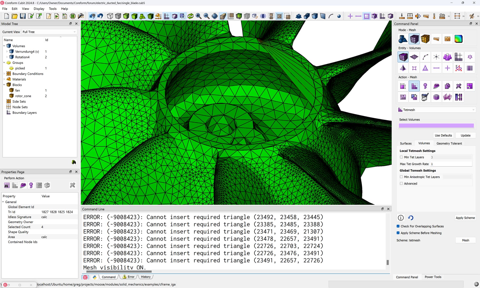
This is so expensive, that for a linear analysis we’d have thrown in the towel and just used a quadratic tetrahedral mesh. Though even this requires a fair bit of manual preprocessing - compositing small surfaces and curves that lead to tet-meshing errors. Even with tet-meshing it’s common that “fire and forget” workflows fall down on complex CAD geometries:
Reviewing traditional meshing
I’ve shared this meshing “journey” to help you better understand the pain that meshing can bring to a finite element analyst. Even though I love Coreform Cubit and am convinced it’s the best meshing experience available, for novices and experts alike, meshing is simply an incredibly difficult problem. Now, with this as our backdrop… let’s look at a better approach… a meshing-free approach with Coreform Flex!
A meshing-free solution with Coreform Flex
Meshing, actually
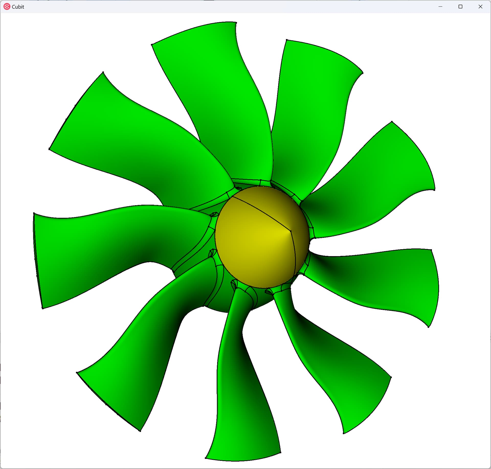
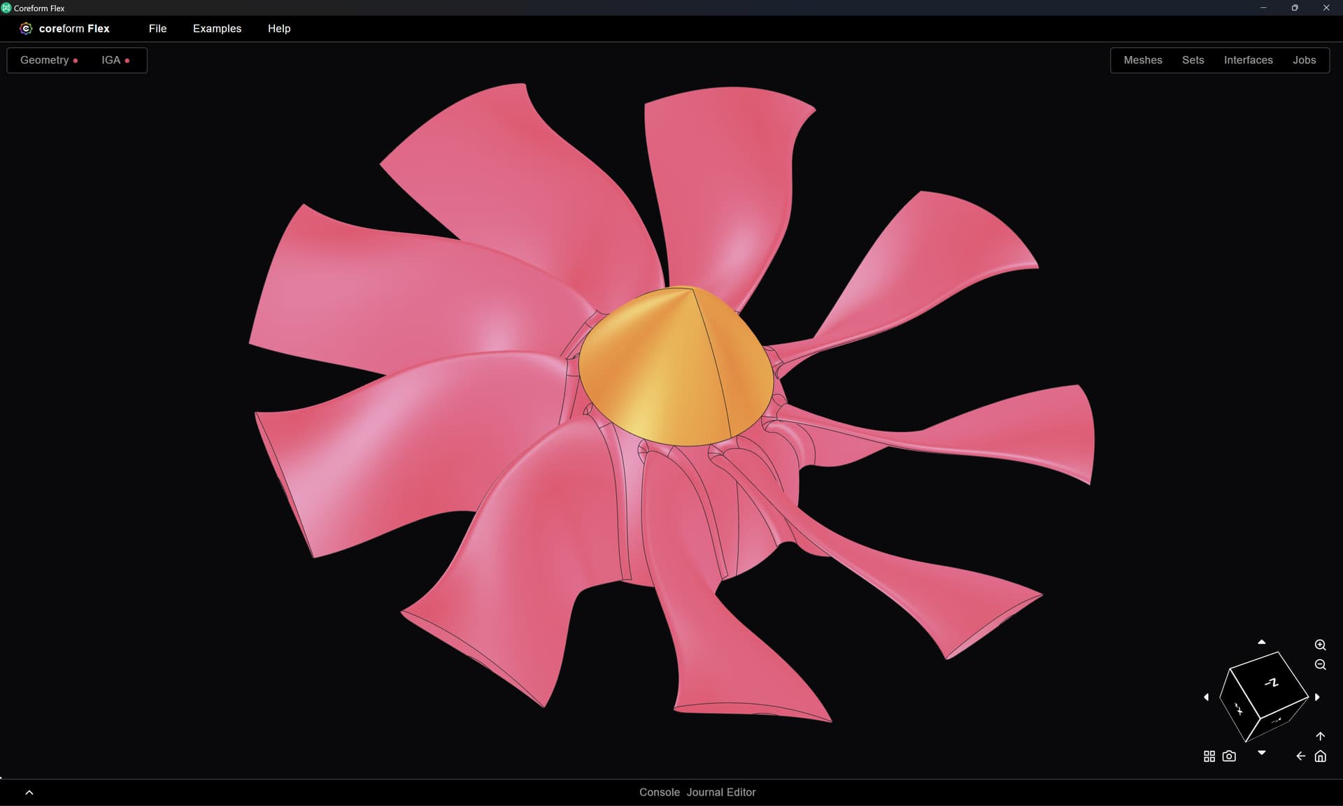
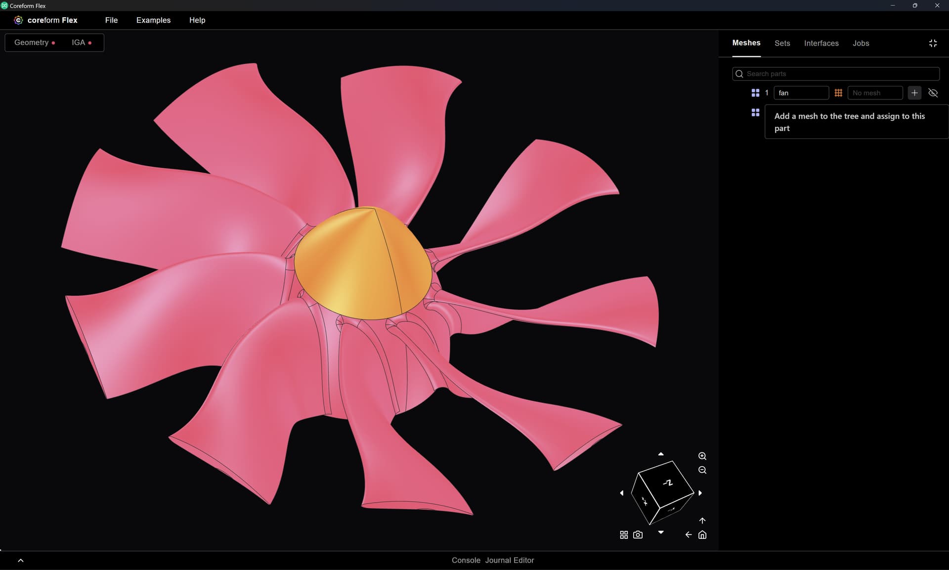
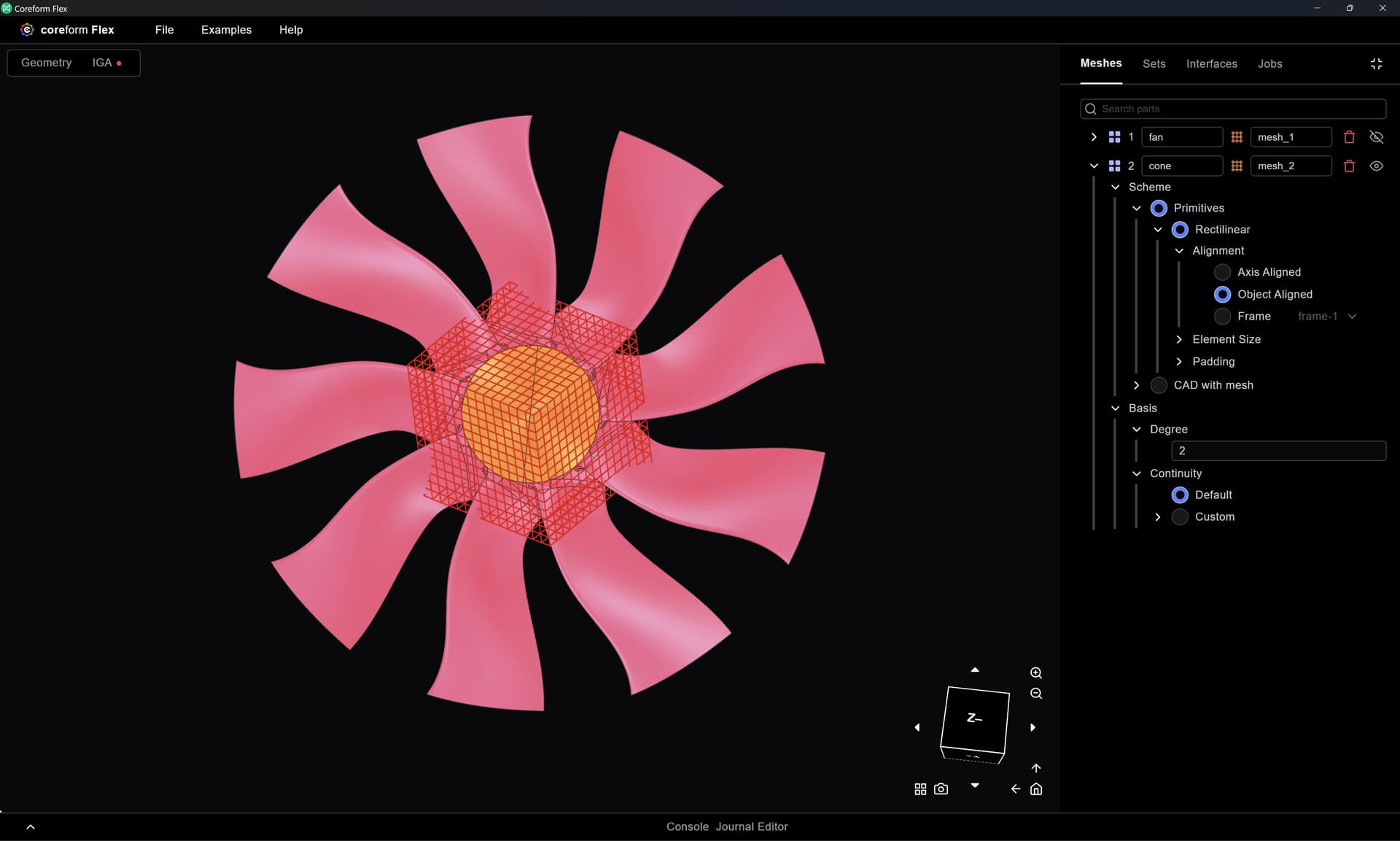
We begin by importing our STEP file into Coreform Flex:
And now let’s mesh the fan by opening the Meshes manager at top right, and then click the + button next to the part named fan (note that just prior, I renamed the two parts from the Deutsch names in the STEP file):
Which produces the following background mesh:
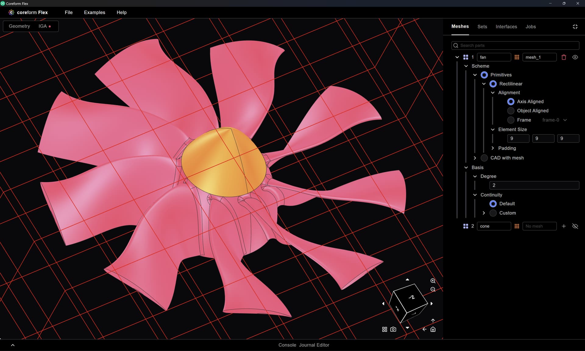
We don’t yet have the best heuristics for the initial mesh size, so we do need to change our mesh size manually.
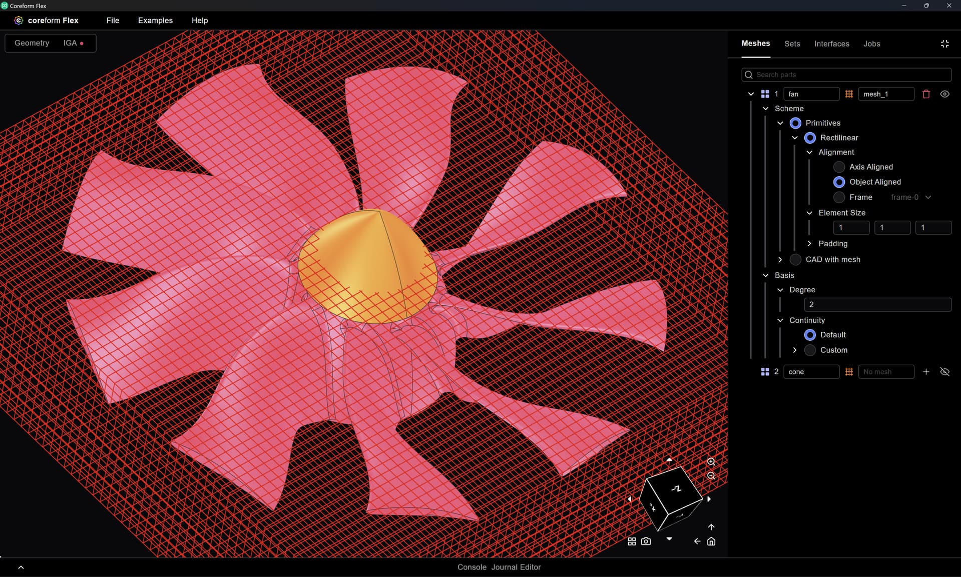
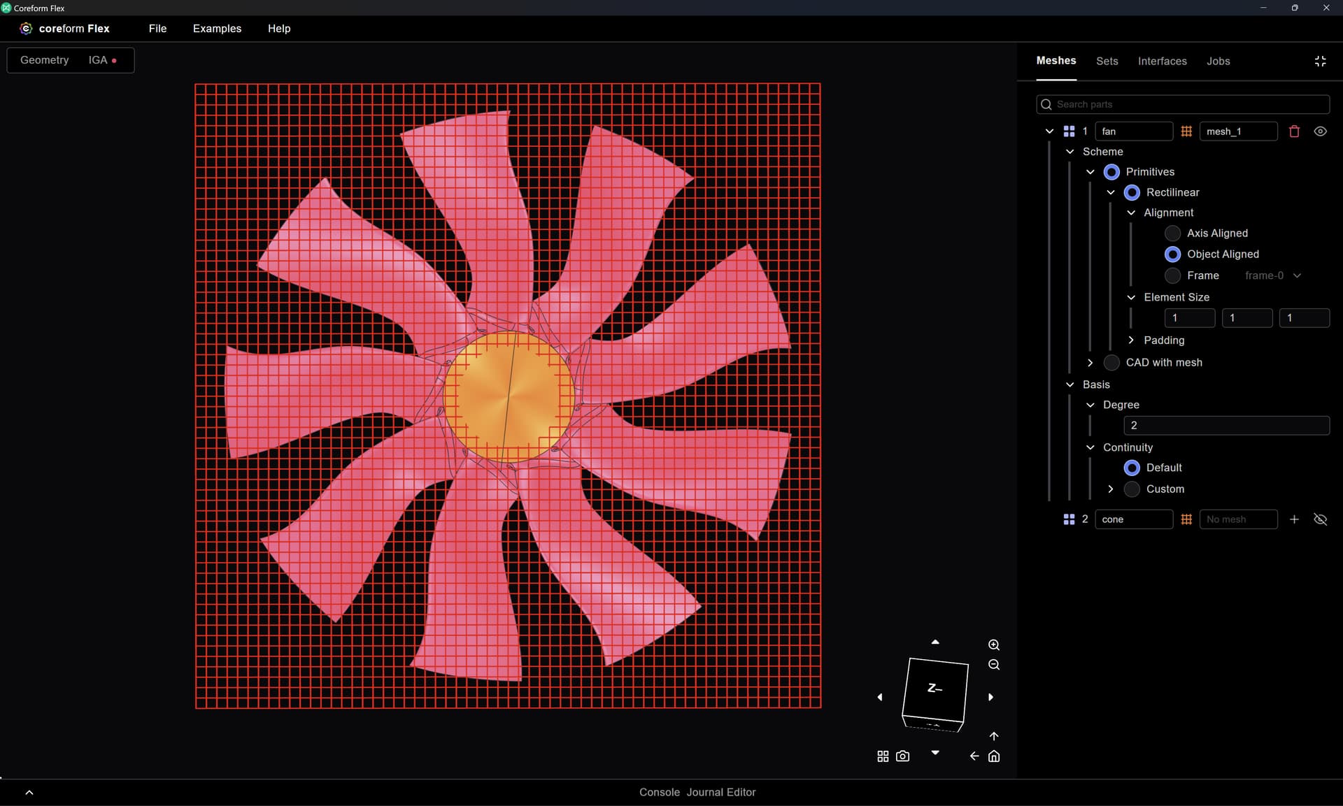
I suppose technically this means we’re still meshing, but recognize that I’ve gone from 40+ hours to produce a mesh on a defeatured fan, to mere seconds to define my mesh on a fully-featured geometry. Next we mesh the cone:
If I want to preview the trimmed mesh that will be computed at simulation submission, I can setup a Trim job in the Jobs manager:
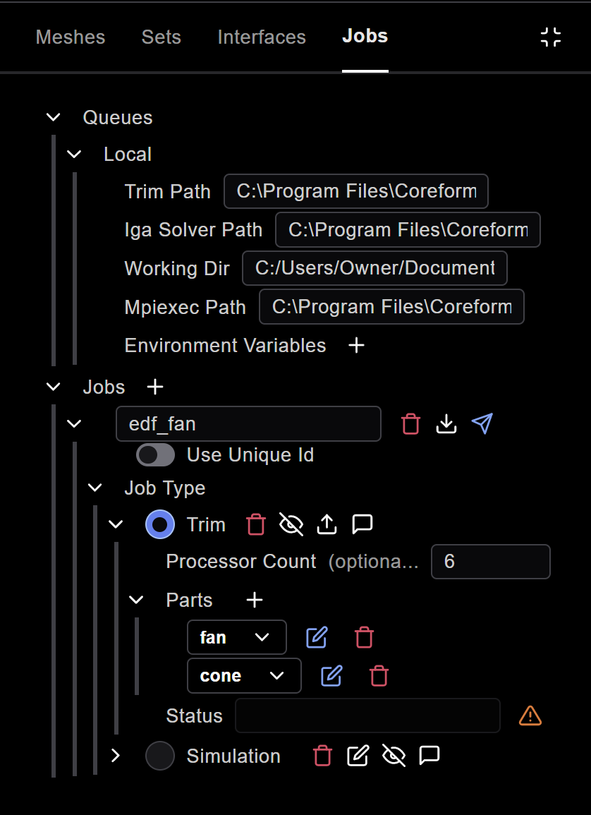
And after the job completes (~4 minutes on my laptop’s 6 cores) click the ![]() icon to render the trimmed mesh:
icon to render the trimmed mesh:
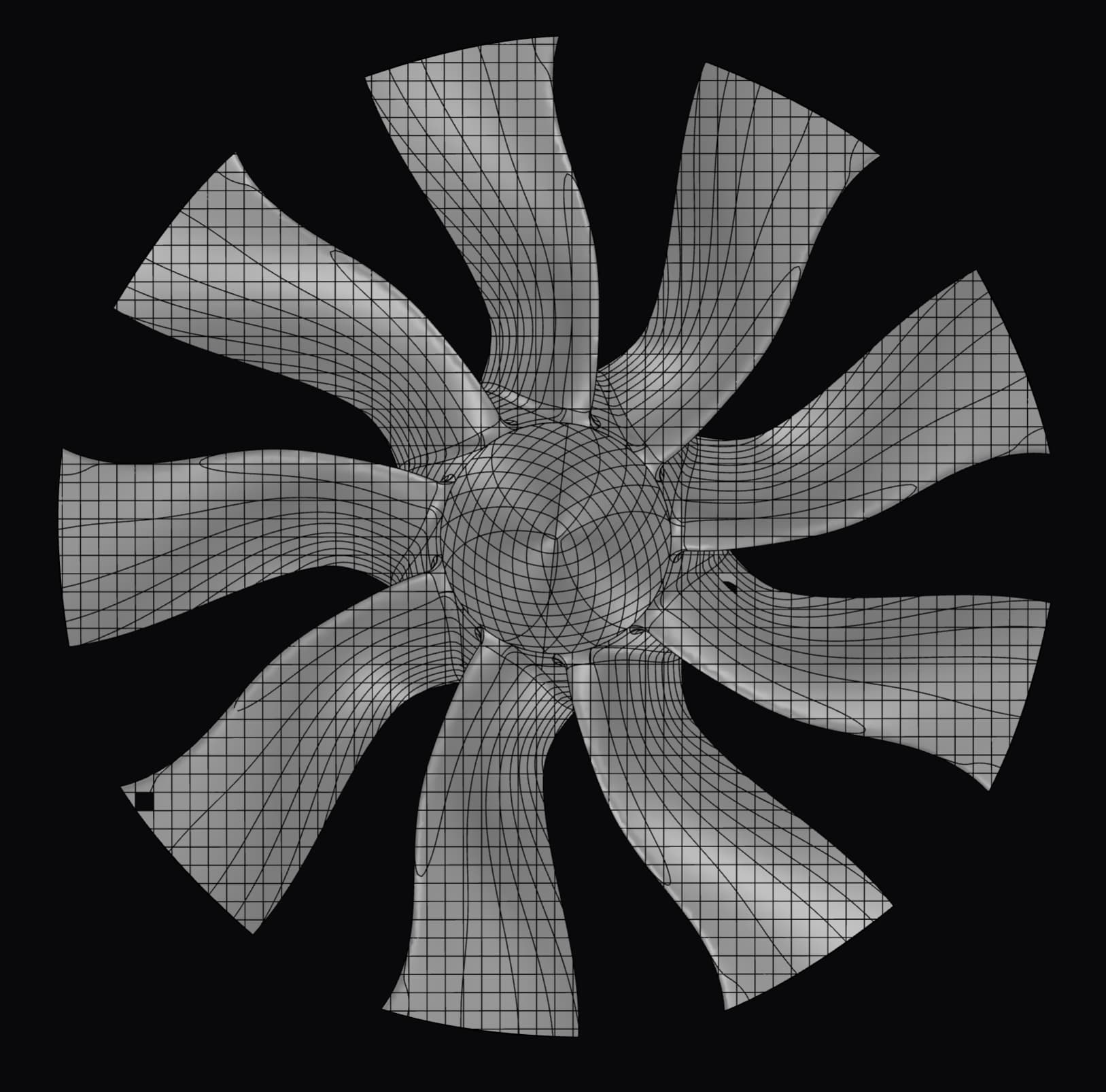
(Note: the missing surfaces - e.g., bottom left - are where we use a fallback scheme that we don’t yet support rendering)
And that’s it, I’m done meshing! Now let’s setup the simulation.
Simulation setup
Our entry-point is through the Procedures object in our IGA model-tree… click the + button
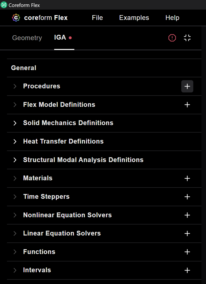
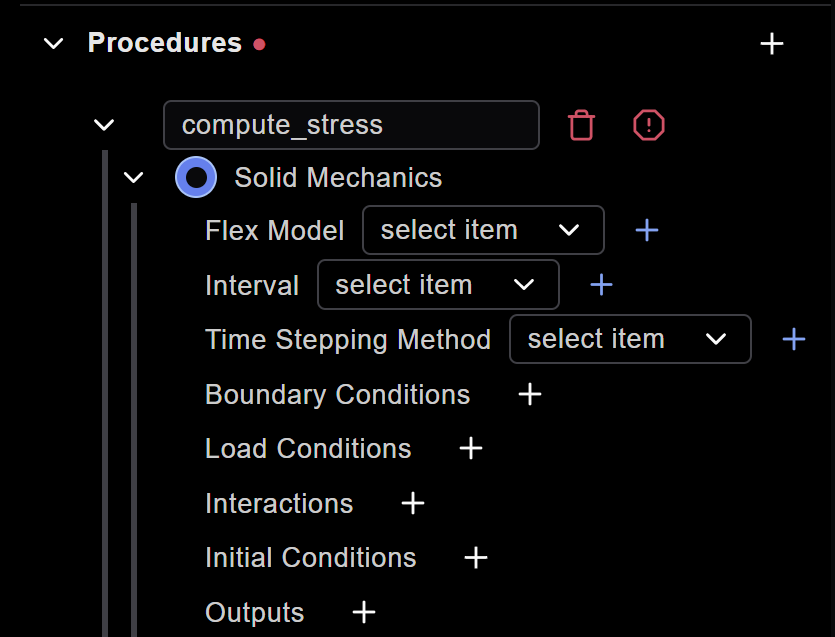
Our goal will be to complete the entries that define our procedure (Currently we only support single-procedure simulations, multi-procedure coming soon!). As we click on the various + buttons, a “breadcrumb” will open that provides a focused view to the model tree.
Creating the Flex Model
We begin by creating our Flex Model – essentially, our simulation assembly:
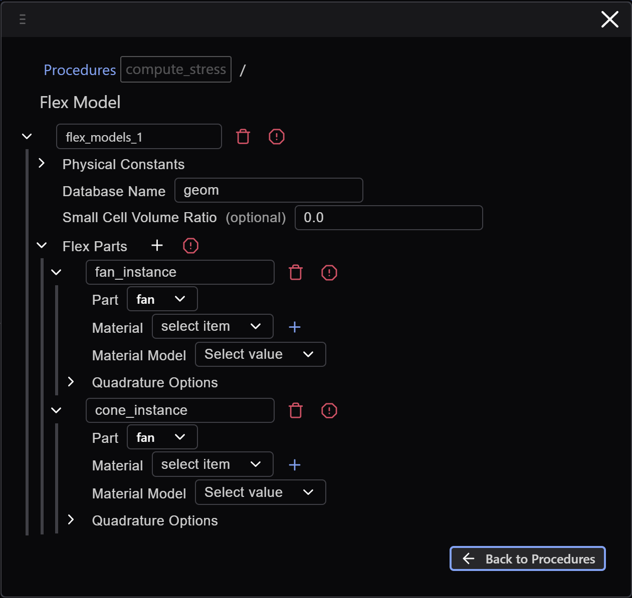
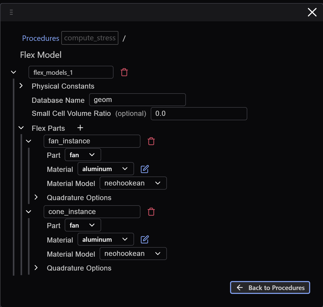
Note that we need to create materials for the analysis (as indicated by the select item text). Clicking the + next to the Material field will take our breadcrumb interface to the material scope, where we create an aluminum material (using the MMTS consistent unit system):

And then, clicking the Back to Flex Model Definitions button we make our selections:
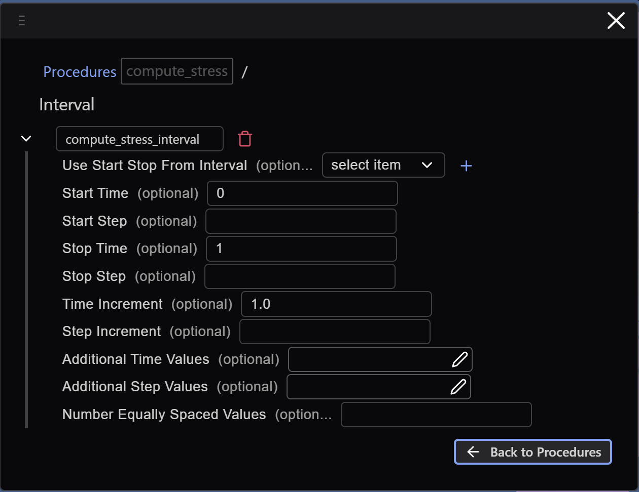
Intervals
We then create an interval for the simulation – we’re going to just perform a linear static analysis, so our “time” interval will be the unit-interval:
Timesteppers
We then create our linear statics timestepper:
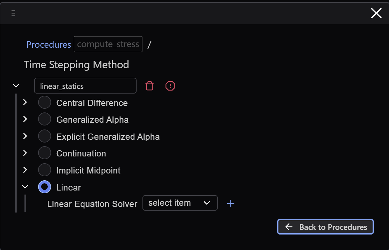
Which needs a linear equation solver:

Boundary conditions
We then create a boundary condition – holding the surfaces at the center of the fan.
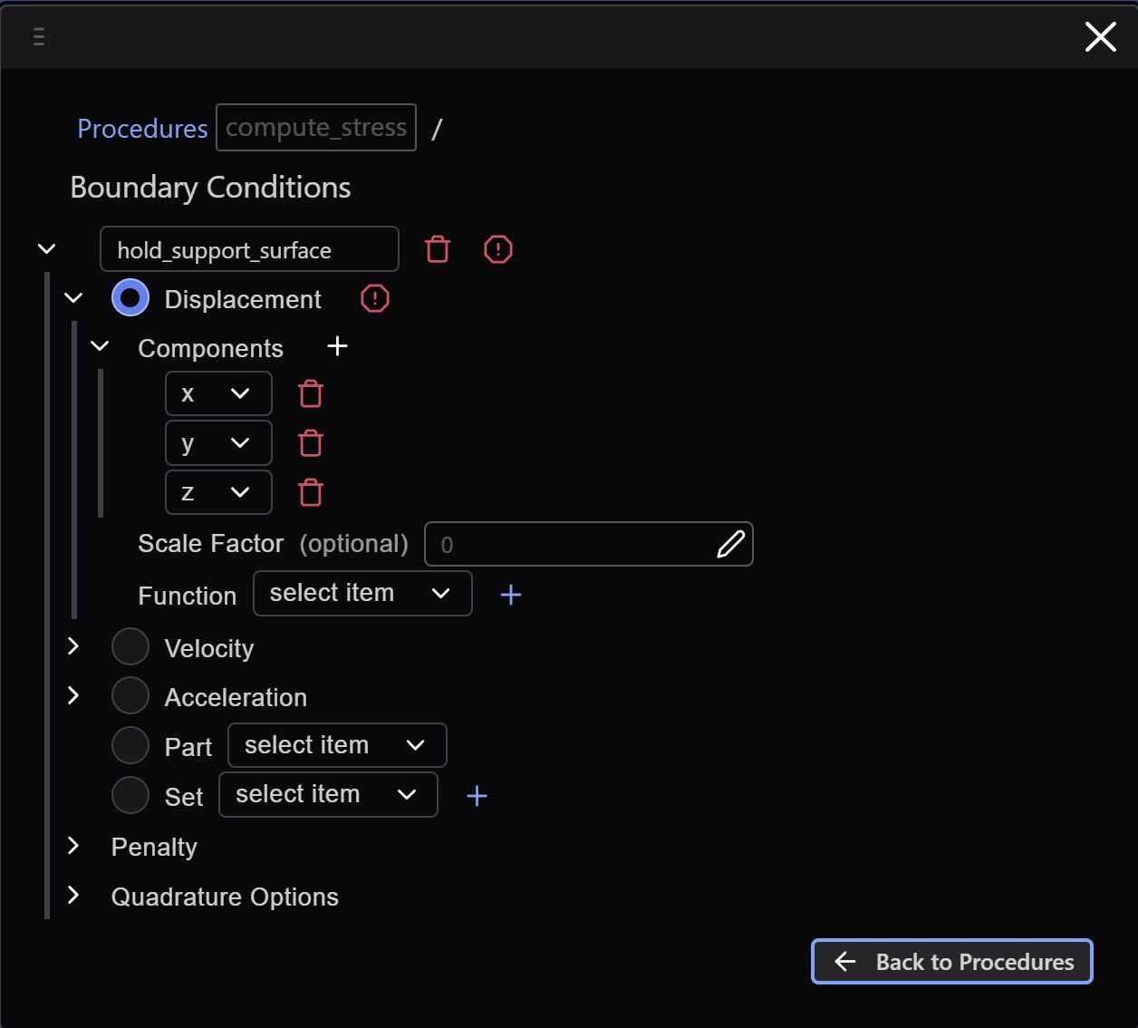
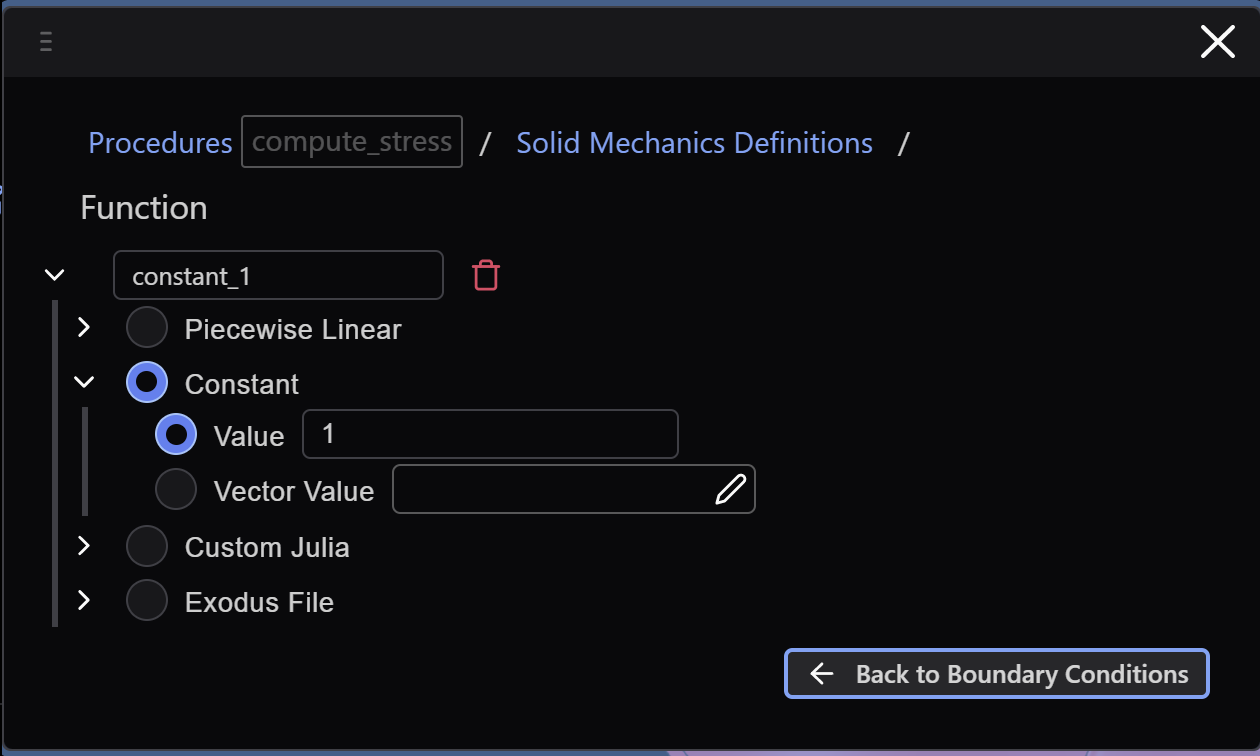
Along the way, we’ll create a function that returns the scalar 1, so that we can then specify a scale_factor = 0 to hold the surfaces fixed:
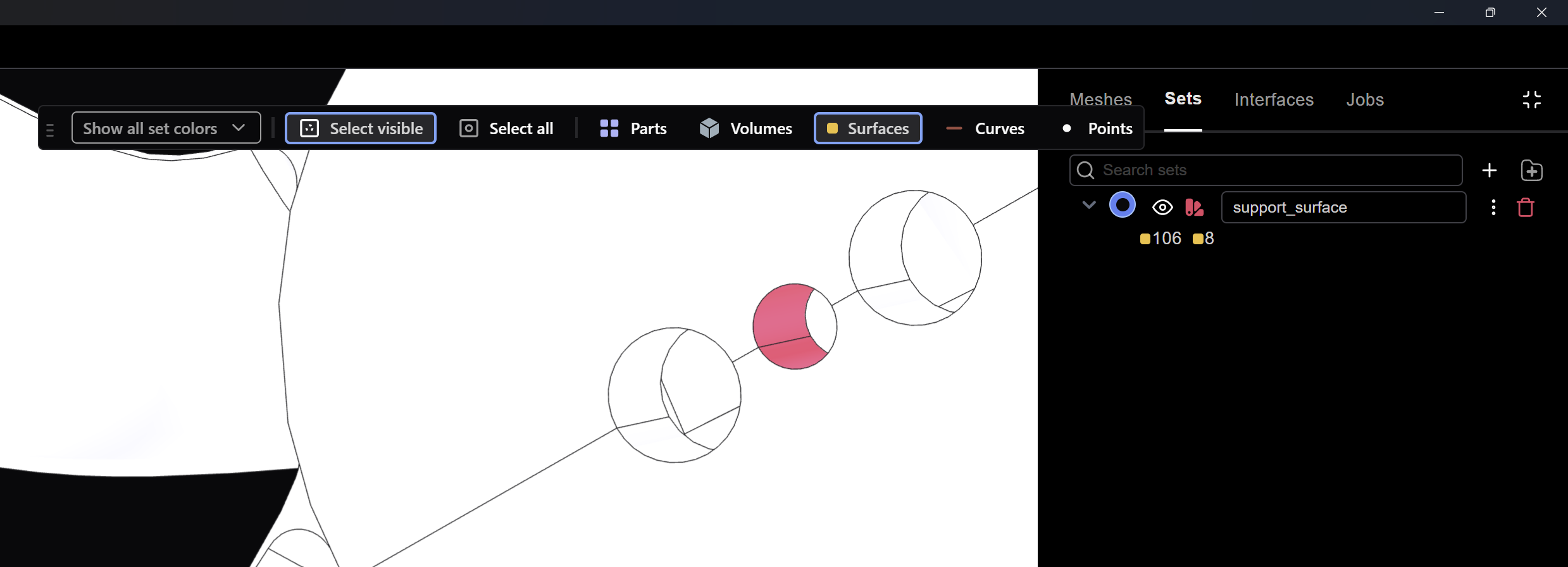
And we need to create a set for our boundary conditions. Clicking the + next to Set will open the Set Manager and we make our selection(s):
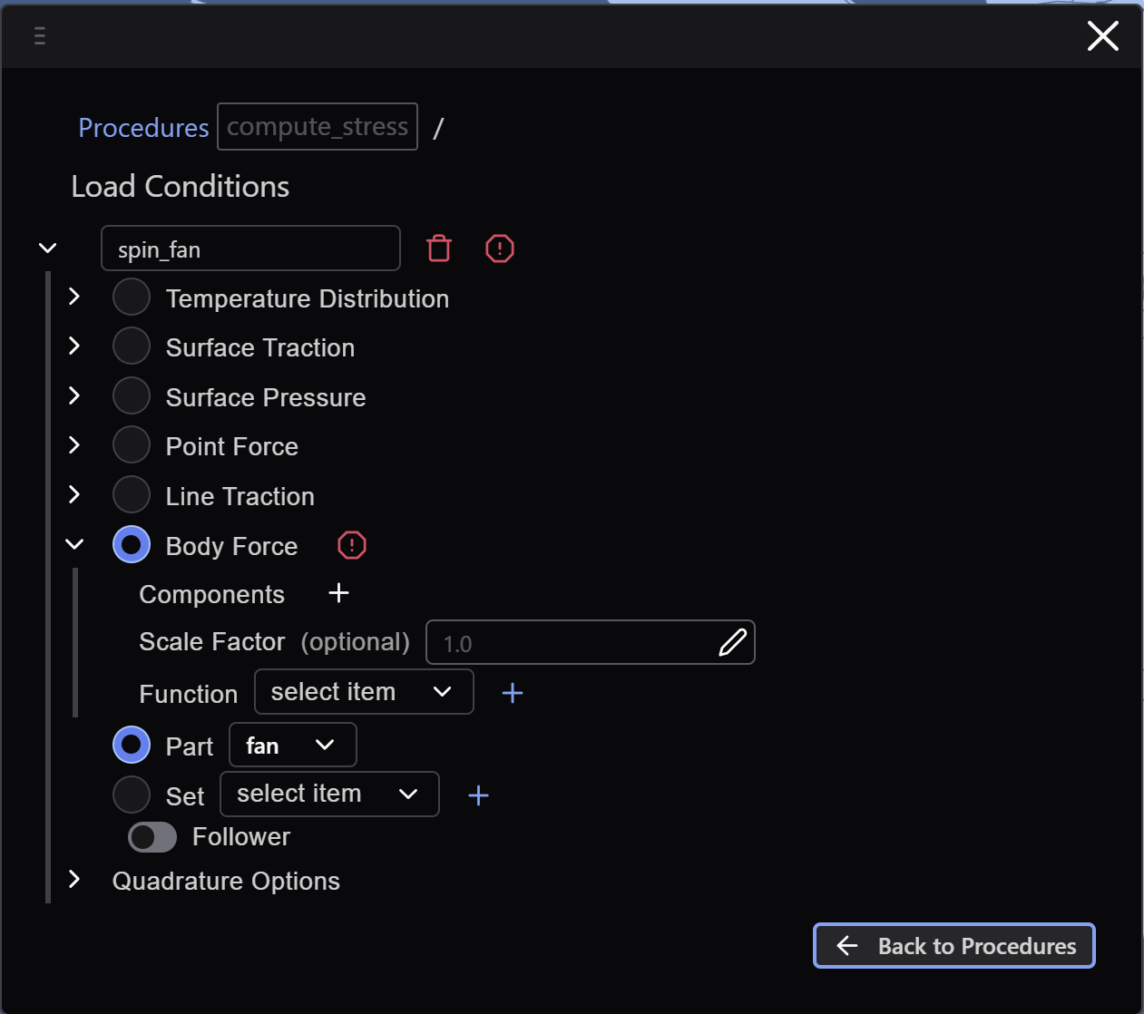
Load conditions
Next we’ll create the centrifugal forces applied to the fan and core. Currently, Coreform Flex doesn’t have a wide variety of available load condition types but we can use a Julia subroutine to define a body force:
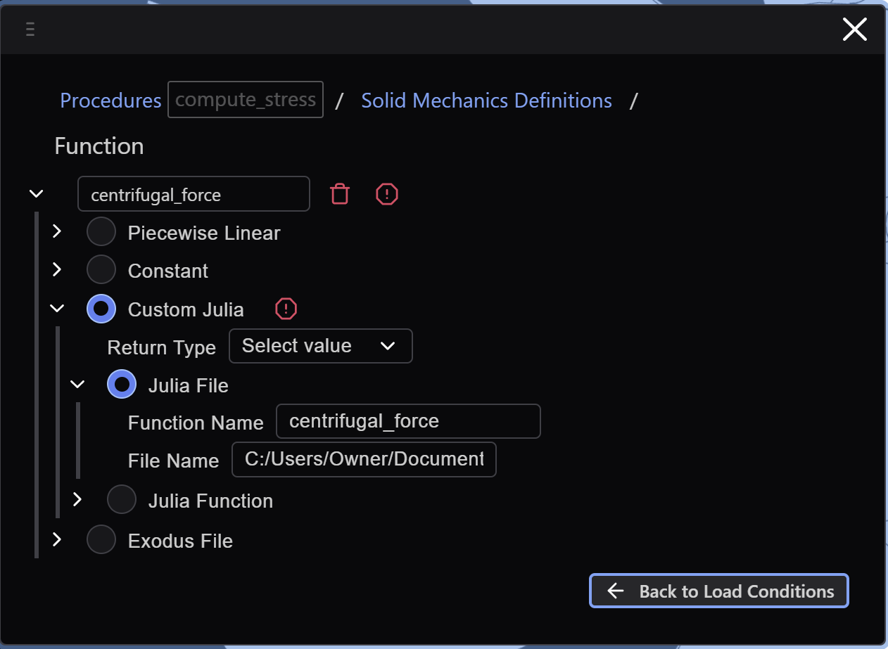
The contents of that Julia file are:
using LinearAlgebra: dot
function centrifugal_force( pos, time )
    mass = 2.712e-9
    ang_vel = 5235.0 # #rad/s -- approx 50,000 RPM
    # Define axis of rotation
    x0 = [ -0.000039, 0.499768, 7.323488]
    x1 = [ 0, 5.257811, -10.433768]
    axis = x1 - x0
    # Project `pos` onto the line defined by x0 and x1
    t = dot( axis, pos - x0 ) / dot( axis, axis )
    # Compute the point on the line
    pos_line = x0 + t * ( axis )
    # Compute the radius vector
    r = pos - pos_line
    return r * mass * ang_vel*ang_vel
end
Interactions
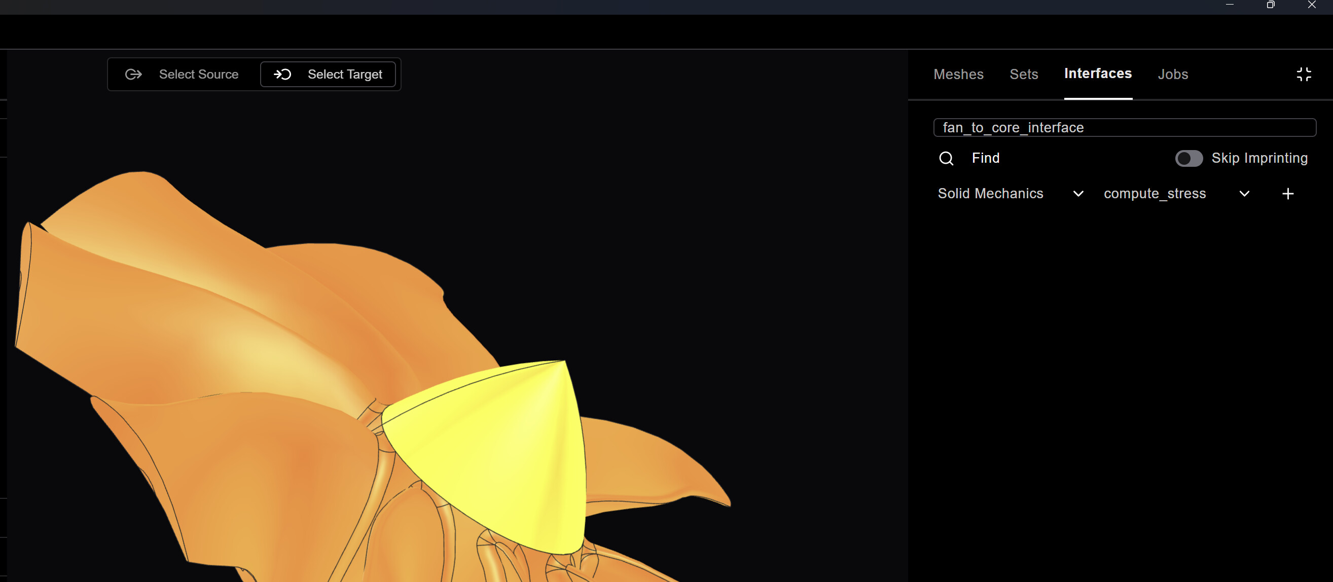
Next we define the connection between the fan and the cone. We will use what we call a material interface – which is the functional equivalent of imprint and merge operations in Coreform Cubit that enforce a contiguous mesh.
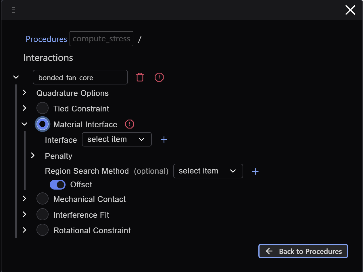
Here, rather than click the + button, let’s define the interface manually in the Interface Manager:
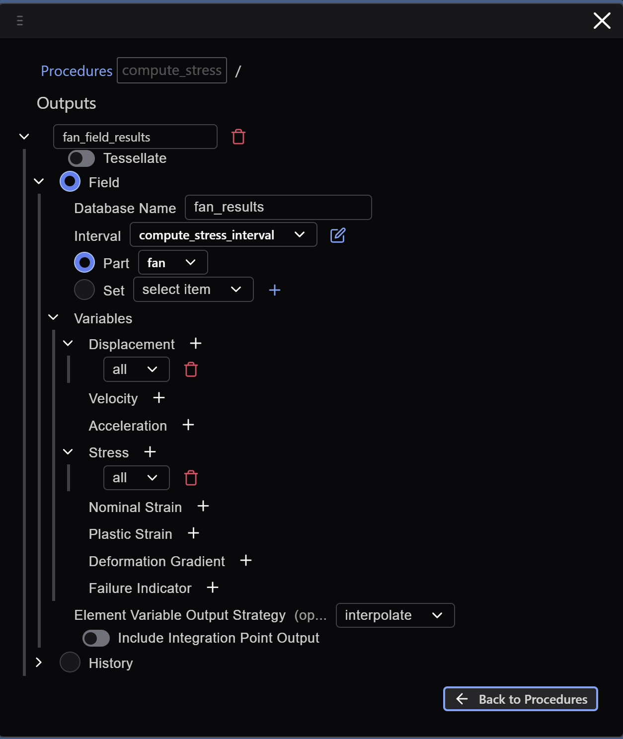
Outputs
And finally, we setup our field outputs:
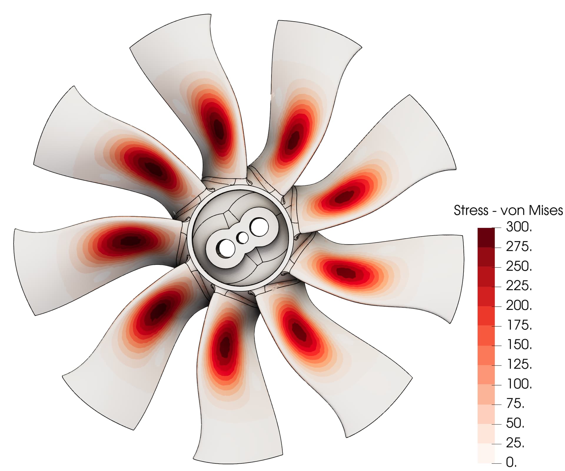
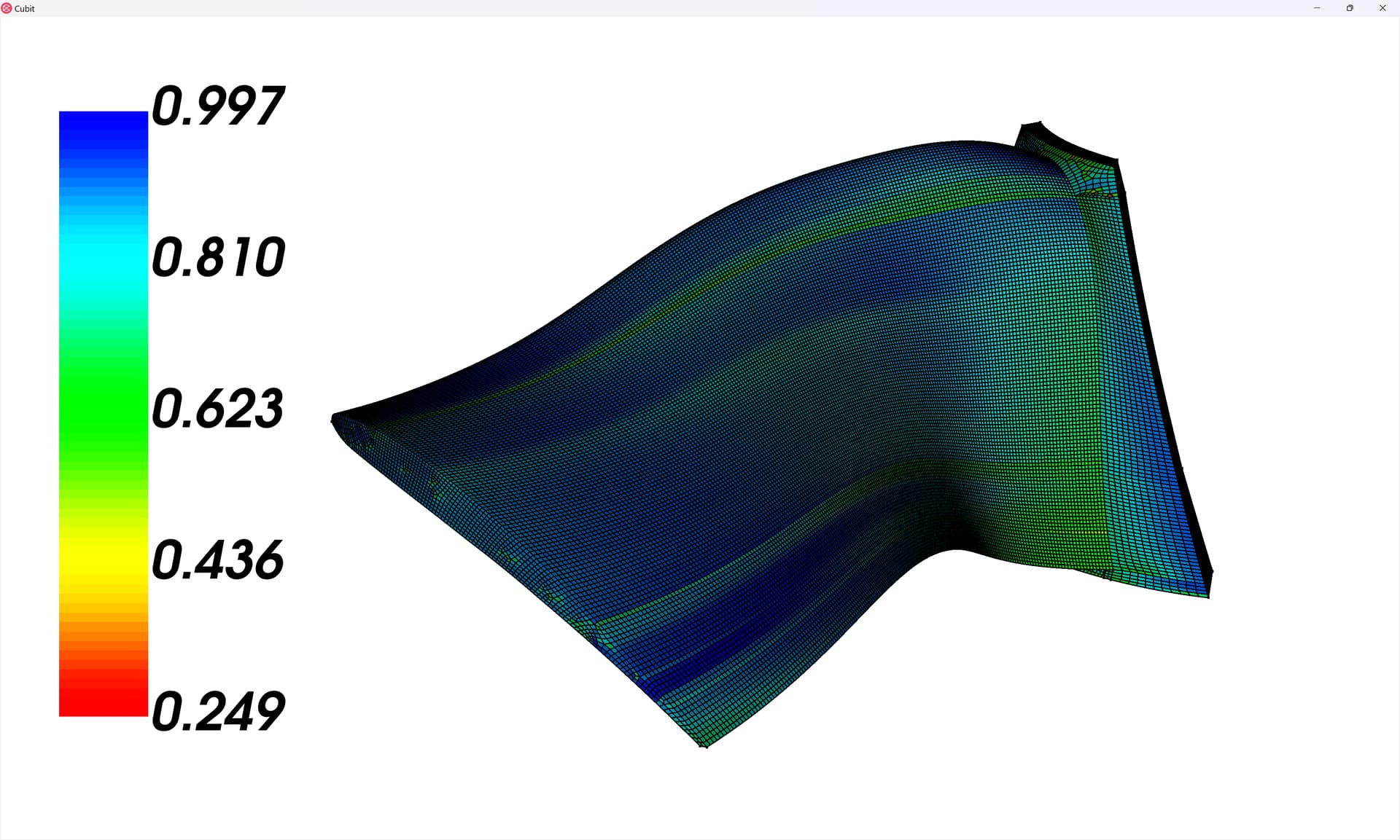
Results
The simulation results can then be visualized using the free, open-source visualization software: ParaView. Below we visualize just the fan component (since the rotor cone’s results aren’t of interest.