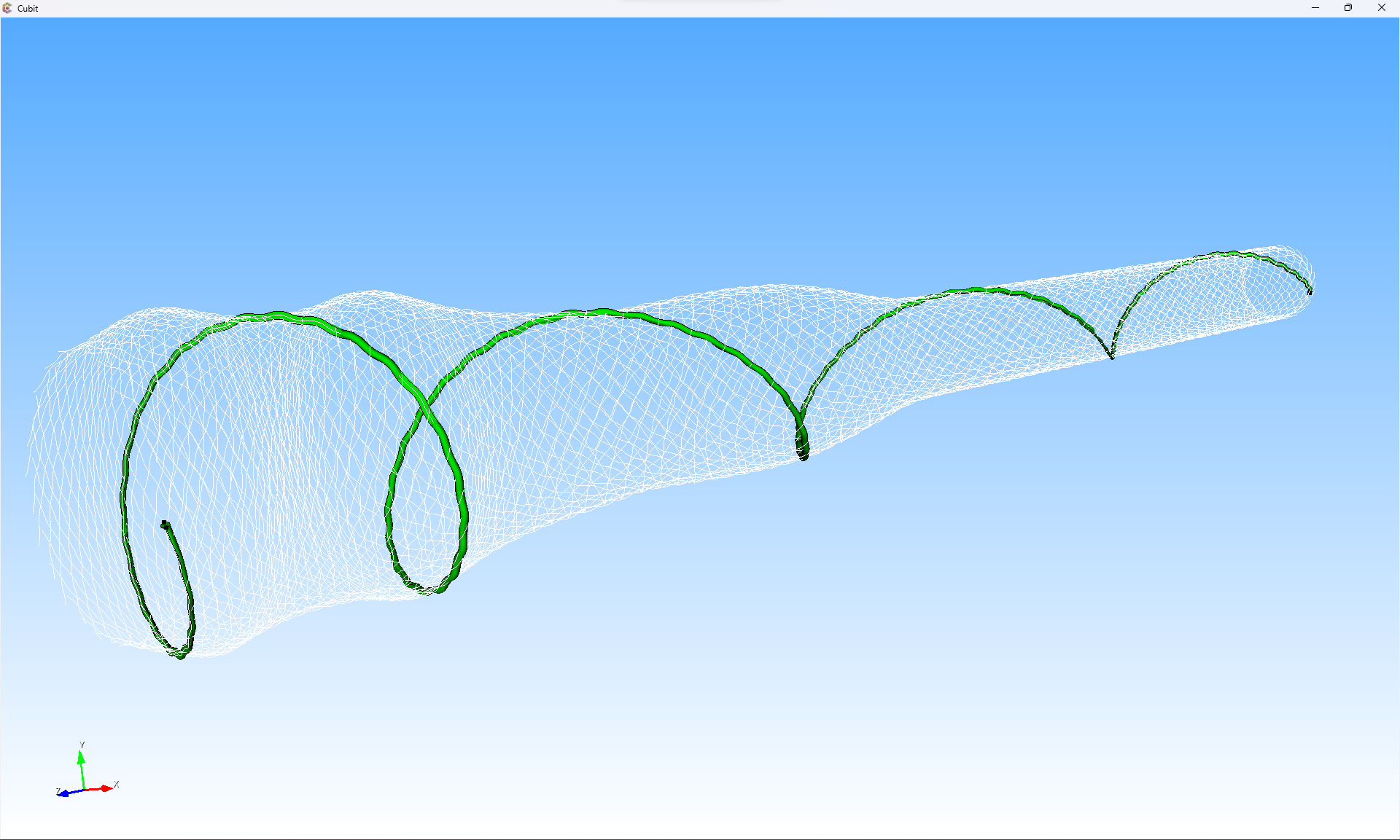
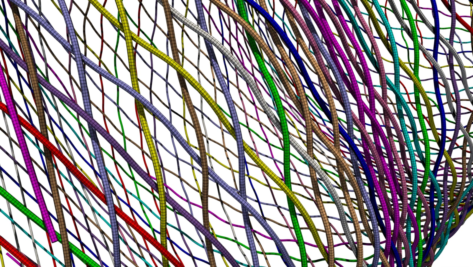
@JeffBodner – here is the completed solution, with a bit of supplemental background information, in the hopes it may be generally insightful for the broader Cubit audience. For those who want to skip the walkthrough, the final script can be downloaded here:
reconstruct_stent_from_mesh.py (4.9 KB)
Background and overview
First, recognize that a mesh consists of two main data structures:
- Element connectivity (topology)
- Nodal coordinates (geometry)
Element connectivity arrays can be represented as a graph which then allows us to make use of various graph theory algorithms. For example, since the node numbers are unordered (the node ids do not increase monotonically from one end to the other), we will compute the ordered arrangement of nodes associated with each wire via the following steps:
- Convert element connectivity array into an undirected graph
- Extract subgraphs representing each wire by computing the connected components of the graph.
- Find the boundary nodes of each wire’s graph
- Compute the simple directed path between the two boundary nodes of each wire’s graph
Then, once we have the path for each wire, we can build a spline through the nodes and sweep a circle along the path.
Installing Python’s networkx package
NetworkX is a Python package for the creation, manipulation, and study of the structure, dynamics, and functions of complex networks and contains data structures for graphs, digraphs, and multigraphs as well as many standard graph algorithms. We will use networkx for the various graph theory algorithms mentioned above but, since it’s not part of the standard Python library we will need to manually install it. In order to use networkx from inside of Coreform Cubit we will need to install it using the Python distributed with Coreform Cubit. To accomplish this on Windows, run the following from a PowerShell terminal:
& 'C:\Program Files\Coreform Cubit 2023.11\bin\python3\python.exe' -m pip install networkx
And in order to use networkx from a separate Python environment you’ll want to do something like:
& 'C:\path\to\your\python.exe' -m pip install networkx
# or
pip install networkx
Main routine
Our main method sets some important Cubit settings to improve performance, before creating the geometry and meshing. Note that on my laptop I can create all the geometry and export the geometry within a couple minutes, but meshing takes ~2-3 hours.
def main():
  # Some default settings for improved performance
  cubit.cmd( "echo off" )
  cubit.cmd( "undo off" )
  cubit.cmd( "warning off" )
  cubit.cmd( "set Default Autosize off" )  # CRITICAL
  # Build the stent geometry and mesh
  cubit.cmd( "reset" )
  load_mesh( filename )
  wire_graphs = generate_wire_graphs()
  generate_wires_from_graph( wire_graphs )
  save_cad()
  mesh_all_wires()
  save_mesh()
Setup script execution
Many Python scripts use the if __name__ == "__main__": statement, here’s how implement it to allow me to run the script either from the Cubit GUI or from an external Python environment.
if __name__ == "__main__":
  import sys
  sys.path.append( r"C:\Program Files\Coreform Cubit 2023.11\bin" )
  import cubit
  main()
elif __name__ == "__coreformcubit__":
  main()
Generate wire graphs
Importing the mesh is straightforward. Note the usage of Python’s f-string functionality, which we will use liberally in this script.
def load_mesh( filename ):
  cubit.cmd( f"import nastran '{filename}'" )
Once we’ve loaded the mesh we can query the mesh connectivity and create the undirected graphs for each wire. In the below routine notice that we initialize an undirected graph for the entire model’s mesh using networkx.Graph(). We can then fill our graph by adding each element as an edge. Then we use networkx.connected_componnents() to get an undirected graph for each wire.
def generate_wire_graphs():
  E = cubit.get_entities( "edge" )
  N = cubit.get_entities( "node" )
  CONN = numpy.zeros( (2,len(E)), dtype="int" )
  CONN_graph = networkx.Graph()
  for e in range( 0, len(E) ):
    eid = E[e]
    CONN[:,e] = cubit.get_connectivity( "edge", eid )
    CONN_graph.add_edge( CONN[0,e], CONN[1,e] )
  components = [ c for c in networkx.connected_components(CONN_graph) ]
  subgraphs = [ CONN_graph.subgraph(c).copy() for c in components ]
  return subgraphs
Generate wires from graphs
This first routine appears a bit superfluous… it loops through each subgraph and generates a wire. However, since each wire creation is fairly expensive, especially if every vertex that we’ll create (there’s ~1000 vertices per wire) is rendered and terminal output printed as each command executes, I’m toggling the graphics on/off and also turning off information output. Note that when you’re running from within Coreform Cubit, Python print() will not print to the terminal.
Also, Cubit has a setting that usually doesn’t have noticeable performance issues, but can cause significant performance issues when working with complex geometries – whenever a geometric entity is created Cubit computes a default mesh size. For these wires it can take several minutes to compute this default size - so we’ll turn it off at the beginning of the script with set Default Autosize off. This does mean that we will need to be sure that we explicitly define mesh sizing later.
def generate_wires_from_graph( subgraphs ):
  for c in range( 0, len( graph ) ):
    print( f"GENERATING WIRE {c+1} OF {len( subgraphs )}" )
    cubit.cmd( "graphics off" )
    cubit.cmd( "info off" )
    generate_wire_from_graph_component( subgraphs[c] )
    cubit.cmd( "graphics on" )
    cubit.cmd( "info on" )
    print( "#"*20 )
This next method is a big one. First notice that I’ve had to write a custom method find_path_order() that will find a node at one end of the wire and then find the node ordering to reach the other end. There’s probably a simpler method in networkx that would do this, essentially computing a path graph, but I couldn’t find a simpler one that worked.
We then create a circular surface, rotate it so that its face-normal aligns to the tangent of the spline at its starting vertex, move it to the starting vertex, and then sweep it along the spline curve to create the wire’s volume. Note my use of the cubit.Dir() object, but I could have used numpy linear algebra routines instead. Then I split the periodic surface of the resulting wire as I suspect it will help with meshing.
def generate_wire_from_graph_component( component ):
  ordered_nodes = find_path_order( component )
  ordered_verts = []
  for nid in ordered_nodes:
    x, y, z = cubit.get_nodal_coordinates( int( nid ) )
    cubit.cmd( f"create vertex {x} {y} {z}" )
    ordered_verts.append( cubit.get_last_id( "vertex" ) )
  cubit.cmd( f"create curve spline location vertex {cubit.get_id_string( ordered_verts )} delete" )
  curve_id = cubit.get_last_id( "curve" )
  curve = cubit.curve( curve_id )
  start_vert_id, stop_vert_id = cubit.parse_cubit_list( "vertex", f"in curve {curve_id}" )
  start_vert = cubit.vertex( start_vert_id )
  cubit.cmd( f"create surface circle radius {radius} zplane" )
  sid = cubit.get_last_id( "surface" )
  face_normal = cubit.Dir( 0, 0, 1 )
  tx, ty, tz = curve.tangent( start_vert.coordinates() )
  orientation = cubit.Dir( tx, ty, tz )
  rot_axis = orientation.cross( face_normal ).get_xyz()
  rot_angle = numpy.rad2deg( orientation.dot( face_normal ) ) + 90
  cubit.cmd( f"rotate Surface {sid} angle {rot_angle} about origin 0 0 0 direction {rot_axis[0]} {rot_axis[1]} {rot_axis[2]}" )
  cubit.cmd( f"move Surface {sid} location vertex {start_vert_id} include_merged" )
  cubit.cmd( f"sweep surface {sid} along curve {curve_id}  keep  individual" )
  vid = cubit.get_last_id( "volume" )
  cubit.cmd( f"split periodic vol {vid}" )
  cubit.cmd( "delete surface all" )
  cubit.cmd( "delete curve all" )
  cubit.cmd( "delete vertex all" )
  cubit.cmd( "compress ids" )
def find_path_order( graph ):
    # Find nodes with valence 1
    endpoints = [node for node in graph.nodes() if graph.degree(node) == 1]
    # Choose one of the endpoints as the starting point for DFS
    start_node = endpoints[0]
    # Perform a depth-first search and get the nodes in order
    ordered_nodes = list( networkx.dfs_preorder_nodes( graph, source=start_node ) )
    return ordered_nodes
Mesh the wires
Meshing the wires uses the same two-method approach I used for creating the mesh geometry, again to allow for some settings modifications and printing progress.
def mesh_all_wires():
  V = cubit.get_entities( "volume" )
  for v in range( 0, len( V ) ):
    print( f"MESHING WIRE {v+1} OF {len( V )}" )
    cubit.cmd( "graphics off" )
    cubit.cmd( "info off" )
    vid = V[v]
    mesh_wire( vid )
    cubit.cmd( "graphics on" )
    cubit.cmd( "info on" )
    print( "#"*20 )
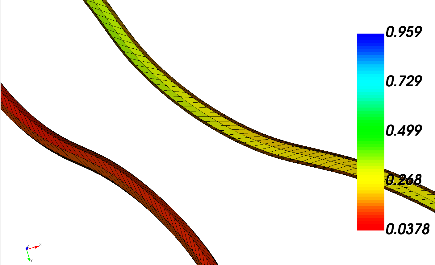
For mesh quality I want to manually specify the sweep meshing scheme for each wire, including specifying a circle mesh scheme on the source surface. The original mesh has some highly skewed elements:
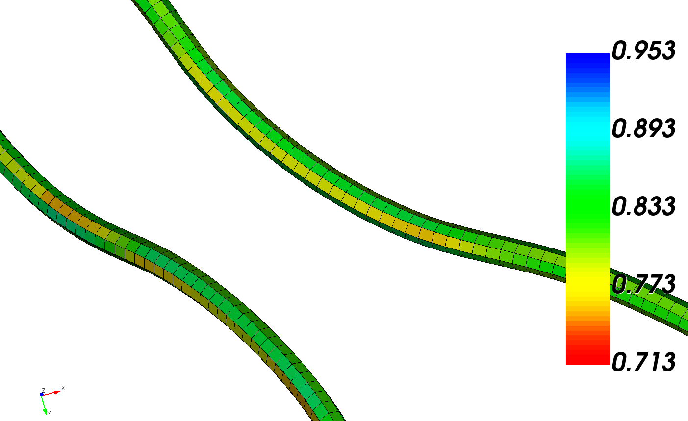
which will improve significantly with the laplacian free volume smooth scheme:
Both the meshing and smooth algorithms are relatively slow due to the expense of evaluating such a large and complicated spline surface - so at least for the smoothing portion I set a pretty loose tolerance of 0.1. It’s also why I split apart the geometry creation routines from the meshing routines.
def mesh_wire( wire_vol_id ):
  vol_surf_ids = cubit.parse_cubit_list( "surface", f"in volume {wire_vol_id}" )
  source_surf_id = None
  target_surf_id = None
  link_surf_ids = []
  for sid in vol_surf_ids:
    if cubit.get_surface_type( sid ) == "plane surface":
      if source_surf_id is None:
        source_surf_id = sid
      else:
        target_surf_id = sid
    else:
      link_surf_ids.append( sid )
  cubit.cmd( f"volume {wire_vol_id} redistribute nodes on" )
  cubit.cmd( f"volume {wire_vol_id} scheme Sweep  source surface {source_surf_id} target surface {target_surf_id} sweep transform translate propagate bias" )
  cubit.cmd( f"volume {wire_vol_id} autosmooth target off" )
  cubit.cmd( f"volume {wire_vol_id} size {radius}" )
  cubit.cmd( f"surface {source_surf_id} scheme circle" )
  cubit.cmd( f"surface {source_surf_id} size {0.7*radius}" )
  cubit.cmd( f"mesh volume {wire_vol_id}" )
  cubit.cmd( f"set smooth tolerance {0.1}" )
  cubit.cmd( f"volume {wire_vol_id} smooth scheme laplacian free" )
  cubit.cmd( f"smooth volume {wire_vol_id}" )
Results
Hopefully this helps demonstrate the use of Cubit’s Python API, and of the wider Python ecosystem, as a pretty powerful tool!